Mathematics E-320 : Teaching Math with a Historical Perspective,

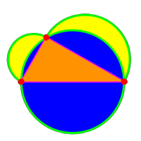
Special Points for Circles

Centroid

(* Proof that the centroid exists, Oliver Knill, January 13, 2010  *)
a={aa,a2,a2};b={b1,b2,b3};c={c1,c2,c3};u=(b+c)/2;v=(a+c)/2;w=(a+b)/2; 
p=(a+b+c)/3;          Simplify[p == a/3+2u/3== b/3+ 2v/3 == c/3+2w/3]

Orthocenter

(* Proof that the orthocenter exists, Oliver Knill, January 13, 2010  *)
a={a1,a2}; b={b1,b2}; c={c1,c2}; 
f[{a_,b_,c_}]:=a+ (b-a)*((c-a).(b-a))/((b-a).(b-a)); 
m=f[{b,c,a}]; n=f[{c,a,b}]; p=f[{a,b,c}];
L[x_,y_,z_,w_]:=x+(t/. Solve[x+t(y-x)==z+s(w-z),{t,s}][[1]])(y-x);
Simplify[ L[a,m,b,n]==L[a,m,c,p]==L[b,n,c,p] ]

Center of Circumscribed Circle

(* Proof that center of the circumscribed circle  exists, Oliver Knill, January 13, 2010  *)
a={a1,a2}; b={b1,b2}; c={c1,c2}; u1=(b+c)/2; v1=(a+c)/2; w1=(a+b)/2; 
p[x_]:={-x[[2]],x[[1]]}; u2=u1+p[c-b]; v2=v1+p[c-a]; w2=w1+p[a-b]; 
L[x_,y_,z_,w_]:=x+(t/. Solve[x+t(y-x)==z+s(w-z),{t,s}][[1]])(y-x);
Simplify[ L[u1,u2,v1,v2]==L[u1,u2,w1,w2]==L[v1,v2,w1,w2] ]

Center of Inscribed Circle

(* Proof that center of the inscribed circle  exists, Oliver Knill, January 13, 2010  *)
a={a1,a2}; b={b1,b2}; c={c1,c2}; 
f[a_,b_,c_] := a+ ((b-a)/Sqrt[(b-a).(b-a)] +(c-a)/Sqrt[(c-a).(c-a)])/2
u=f[a,b,c]; v=f[b,c,a]; w=f[c,a,b]; 
L[x_,y_,z_,w_]:=x+(t/. Solve[x+t(y-x)==z+s(w-z),{t,s}][[1]])(y-x);
Simplify[ L[a,u,b,v]==L[a,u,c,w]==L[b,v,c,w] ]

Feuerbach proof

(* Proof that the 9 point circle exists, Oliver Knill, January 13, 2010  *)

LineIntersect[A1_,A2_,B1_,B2_]:= A1 + (t /. Solve[A1+t (A2-A1) == B1+s (B2-B1),{t,s}][[1]]) (A2-A1);
BasePoint[a_,b_,c_]:=a+(b-a) ((c-a).(b-a)/((b-a).(b-a)));      MidPoint[a_,b_]:=(a+b)/2;
Umkreis[a_,b_,c_]:=Module[{R,n1,n2,center,radius},{x1,y1}=a;{x2,y2}=b;{x3,y3}=c;
  R = 2*(x3*(y1-y2)+x1*(y2-y3) + x2*(-y1 + y3));
  n1=(x3^2*(y1-y2)+(x1^2+(y1-y2)*(y1-y3))*(y2-y3)+x2^2*(-y1+y3))/R;
  n2=(-(x2^2*x3)+x1^2*(-x2+x3)+x3*(y1^2-y2^2)+x1*(x2^2-x3^2+y2^2-y3^2)+x2*(x3^2 - y1^2+y3^2))/R;
  center={n1, n2};radius=(center-a).(center-a); {center,radius}];

p1={px1,py1}; p2={px2,py2}; p3={px3,py3};
m3 = MidPoint[p1,p2]; m2 =MidPoint[p1,p3]; m1 = MidPoint[p2,p3];
h3 = BasePoint[p1,p2,p3]; h1=BasePoint[p2,p3,p1]; h2=BasePoint[p3,p1,p2];
m  = LineIntersect[p1,h1,p2,h2]; q1=MidPoint[m,p1]; q2=MidPoint[m,p2]; q3=MidPoint[m,p3];
Simplify[Umkreis[q1,q2,q3]==Umkreis[m1,m2,m3]==Umkreis[h1,h2,h3]]

Fermats Last Theorem

These numbers appear in the Simpsons Epiosode Treehouse of horror.

N[(1782^12 + 1841^12)^(1/12)]

Andrica Conjecture

The conjecture tells that the differences between the squareroots of consecutive primes is always smaller than 1.

Andrica[n_]:=Sqrt[Prime[n+1]] - Sqrt[Prime[n]];
ListPlot[Table[Andrica[n],{n,1,10000}],PlotRange->All]

Gilbreaths Conjecture

s0= Table[Prime[n],{n,1,10}]
diff[s_]:=Append[Table[s[[n+1]]-s[[n]],{n,Length[s]-1}],0]
NestList[diff,s0,Length[s0]];

Solving the Cubic

The depressed Cubic x³+px+q can be reduced to a quadratic equation by a substitution. First remove the quadratic part with X=x-a/3 so that X³²+bX+c becomes the depressed version x³ + p x + q. Now substitute x=u-p/(3u) to get a quadratic equation (u⁶+qu³-p³/27)/u³=0.

X = x-a/3; X^3 + a X^2 + b X + c
x = u - p/(3 u); Simplify[u^3*Expand[ x^3 + p x + q]]

Schwarz Paradox

r=7; h=10; n=10; m=5;
P = Table[ {Cos[2 Pi k/n],Sin[2 Pi k/n],l/m},      {k,1,n},{l,1,m}];
Q = Table[ {Cos[2 Pi (k+1/2)/n],Sin[2 Pi (k+1/2)/n],(l+1/2)/m},{k,1,n},{l,1,m}];
U = Table[ {Cos[2 Pi (k+1/2)/n],Sin[2 Pi (k+1/2)/n],(l+1/2)/m},      {k,1,n},{l,1,m}];
V = Table[ {Cos[2 Pi (k+1)/n],Sin[2 Pi (k+1)/n],(l+1)/m},{k,1,n},{l,1,m}];
S1 = {RGBColor[1,1,0],Table[ Polygon[{P[[k,l]],Q[[k,l]],P[[Mod[k,n]+1,l]],P[[k,l]]}],{k,1,n},{l,2,m}]};
S2 = {RGBColor[1,0.5,0],Table[ Polygon[{P[[k,l]],Q[[k,l-1]],P[[Mod[k,n]+1,l]],P[[k,l]]}],{k,1,n},{l,2,m}]};
S3 = {RGBColor[0,1,1],Table[ Polygon[{U[[k,l]],V[[k,l]],U[[Mod[k,n]+1,l]],U[[k,l]]}],{k,1,n},{l,1,m}]};
S4 = {RGBColor[0.5,1,1],Table[ Polygon[{U[[k,l]],V[[k,l-1]],U[[Mod[k,n]+1,l]],U[[k,l]]}],{k,1,n},{l,2,m}]};
S=Show[Graphics3D[{S1,S2,S3,S4}], Boxed->False, SphericalRegion->True,Background->RGBColor[0,0,1]];

Expected win in Petersburg Casino

The function F[w] computes the expected win using an utility function which depends on the W richness of the player. As richer the player is as more he or she can bet to get even.

F[W_]:=Module[{},L=1+Floor[Log[2,W]]; L/2 + W/2^L];

Dynamical systems

The Mandelbrot set

M=Compile[{x,y},Block[{z=x+I y,k=0},While[Abs[z]<2&&k<50,z=z^2+x+I y;++k];k]];
DensityPlot[50-M[x,y],{x,-2.,1.},{y,-1.5,1.5},PlotPoints->200,Mesh->False];

The Julia set with c=-0.12+0.74 i is the Douady rabbit. 
J=Compile[{u,v},Block[{z=u+I*v,k=0},While[Abs[z]<99&&k<50,z=z^2-.12+.74I;++k];k]];
DensityPlot[50-J[u,v],{u,-1,1},{v,-1,1},PlotPoints->200,Mesh->False];


Game of life

SizeOfWorld=50; M=SizeOfWorld; x=Table[Random[Integer,1],{M},{M}]; 
m[k_]:=Mod[k-1,M]+1;
Do[y=Table[x[[m[i+1],j]]+x[[m[i-1],j]]+x[[i,m[j+1]]]+x[[i,m[j-1]]]+
           x[[m[i-1],m[j-1]]]+x[[m[i-1],m[j+1]]]+
           x[[m[i+1],m[j-1]]]+x[[m[i+1],m[j+1]]],{i,M},{j,M}];
   Do[Do[If[x[[i,j]]==1, If[Abs[y[[i,j]]-2.5]>1,x[[i,j]]=0],
         If[y[[i,j]]==3, x[[i,j]]=1]],{i,M}],{j,M}];
   ListDensityPlot[1-x,Mesh->False,Axes->False],{k,10}]



Cellular Automata

M=100;V=CellularAutomaton[18,Table[Random[Integer,1],{k,M}],M];
ListDensityPlot[Reverse[V],Mesh->False,Frame->False,Axes->False]


Lorentz attractor:
Lorentz=NDSolve[{x'[t]==10(y[t]-x[t]),y'[t]==-x[t] z[t]+28x[t]-y[t],
z'[t]==x[t]*y[t]-8z[t]/3,x[0]==z[0]==0,y[0]==.3},{x,y,z},{t,0,40},MaxSteps->5000];
ParametricPlot3D[Evaluate[{x[t],y[t],z[t]}/. Lorentz],{t,0,40}, PlotPoints->5000];


The riddle: 
T[x_]:=4 x (1-x); A=NestList[T,0.3,100];
S[x_]:=4 x -4x^2; B=NestList[S,0.3,100];
ListPlot[A-B]


Drawing bifurcation diagrams
g=Compile[{c},({c,#} &) /@ Union[Drop[NestList[c*#(1-#) &,0.3,500],400]]];
s=Table[g[c],{c,2.5,4,0.0001}];
ListPlot[Flatten[s,1],PlotStyle->{AbsolutePointSize[.0001]}]


Cobweb construction:

T[x_]:=4 x(1-x); o={{0.3,T[0.3]}}; p={{0.3,0},{0.3,T[0.3]}};
Do[l=Last[Last[o]]; o=Append[o,{l,l}]; o=Append[o,{l,T[l]}],{8}];
Show[Plot[{T[x],x},{x,0,1}],Graphics[{Line[p],Line[o]}]];


Henon attractor
T[{x_,y_}]:=N[{1-1.4*x^2+y,0.3*x}];
S[p_]:=T[p];c=Last[NestList[S,{0,0},300]]; F=NestList[S,c,100000];
G[R_]:=ListPlot[F,PlotRange->R,PlotStyle->{PointSize[10^(-6)]}];
Do[G[{{c[[1]]-2^k,c[[1]]+2^k},{c[[2]]-2^k,c[[2]]+2^k}}],{k,-6,0}];