The Boolean-Green function problem

In
unit 6, you explored the question whether the inverse of
an invertible n x n matrix with entries 0 or 1 always has entries 0,1,-1 (as in the
case n=2. The answer is already ``no" in the case n=3, but only in the case n=4
is it possible that the maximal entry is larger than 1, like 2. Matrices with entries 0 or 1
are also called
Boolean matrices. They are of great interest in mathematics. Now, we can ask:
|
How large can A-1ij get if A is an invertible nxn Boolean matrix?
|
I call it the
Boolean Green function problem.
In principle, we can look over the entire set of all 0-1 matrices, but that set is getting large
pretty quickly. It can still just be done for n=5, where we have 2
25=33554432 matrices (this is the
last value, where I could get through all cases and confirm the maximum).
For n=6, we would have to run through 2
36 = 68719476736 matrices already. Anyway,
here is the code to check it all. Try to change 3 to 7 and see your laptop burn! You would
need Thousands of TBytes of Ram just to evaluate Boolean[7] which consists of
562'949'953'421'312 matrices.
Boolean[n_]:=Tuples[{0,1},{n,n}];
F[n_]:=Module[{B=Boolean[n]},
Max[Table[If[Det[B[[k]]]!=0,
   Max[Flatten[Inverse[B[[k]]]]],0],
    {k,Length[B]}]]];
F[3]
|
Monte Carlo tests
For n=20 already, we have 2
400 ∼ 10
120 possibilities. There are about 10
80
elementary particles in the observable universe so that this is not an option even if each particle would
have computed a zillion of case each second since the big bang (10
17 seconds in the past).
But we can explore using
Monte-Carlo tests, producing random matrices and see how large values we can
get by probing the large space. This might well miss the actual maximum as the maxima become
needles in a haystack
but probing the space randomly could give us an idea about the growth:
RandomInvertibleBooleanMatrix[n_]:=Module[{A,found=False},
  While[Not[found],A=Table[Random[Integer,1],{n},{n}];
                    found=(Det[A]!=0)];A];
FindExtrema[n_,tries_]:=Module[{max=1,min=1,M,m},
  Do[A=RandomInvertibleBooleanMatrix[n];
     M=Max[Flatten[Inverse[A]]]; If[M>max,max=M; Print[max]];
     m=Min[Flatten[Inverse[A]]]; If[min>m,min=m; Print[min]],
  {tries}]; {min,max}];
Do[ Print[{n,N[FindExtrema[n,100000]]}],{n,1,12}]
|
The maxima and minima grow as follows. For values like n=11,12 we run the experiment for hours
to get the larger values. The value min(11)=-135 soon no more extremal. One can bet there is a
value -141 too. We let it run for a weekend (actually, the value 148 just appeared on Sunday
(Feb 17, 2019) 151 on Monday Feb 18, 2019, so that also 141 was not the maximum yet.
Monday also gave 83 for n=10.) The Boolean spaces of matrices are just too huge
and the cases with maximal value too sparse to reach in a reasonable time.
n   = {1, 2, 3, 4, 5, 6, 7,  8,  9, 10, 11,   12  }
min = {1,-1,-1,-2,-3,-5,-9,-18,-39,-80,-156,-213  }
max = {1, 1, 1, 2, 3, 5, 9, 18, 38, 94, 151, 213  }
       *  *  *  *  *
       true  values  |  records so far
|
Updates:
- ran n=11 for a weekend: record instead of -135 to -156 and 148 instead of 141
- ran n=10 also longer: instead of 62 record -80 and 80 now
- n=9 -> 38, n=10 -> 83, n=11 -> 151 , n=9 -38 -> -39
- Feb 21: n=10 -> 94
Obviously, the numbers max(n) and min(n) change monotonically: we can look at the partitioned matrix, where
one matrix is a 1x1 matrix and the other a (n 1) x (n-1) matrix. A maximum or minimum for
n-1 can now be matched also for n. Note that the Green function entries are not integers in
general. They are rational. But the maximum and minimum appear to be integers. We experimentally
see that this is the case when the determinant is 1 or -1, which is when the Boolean matrix is
unimodular. One can use geometry to generate matrices with large Green function entries. The
unimodularity theorem
assures that the Boolean matrix encoding the intersections of sets in a
finite abstract simplicial complex is always unimodular. The maximal Green function entries are
there geometric.
|
Conjecture: The minimum and maximum Green function value is an integer
|
|
Conjecture: The minimum is minus the maximum.
|
This is so far supported by the fact that in the above numbers,
when we saw a difference, we just ran the code again for much longer time
to find the lower or higher numbers.
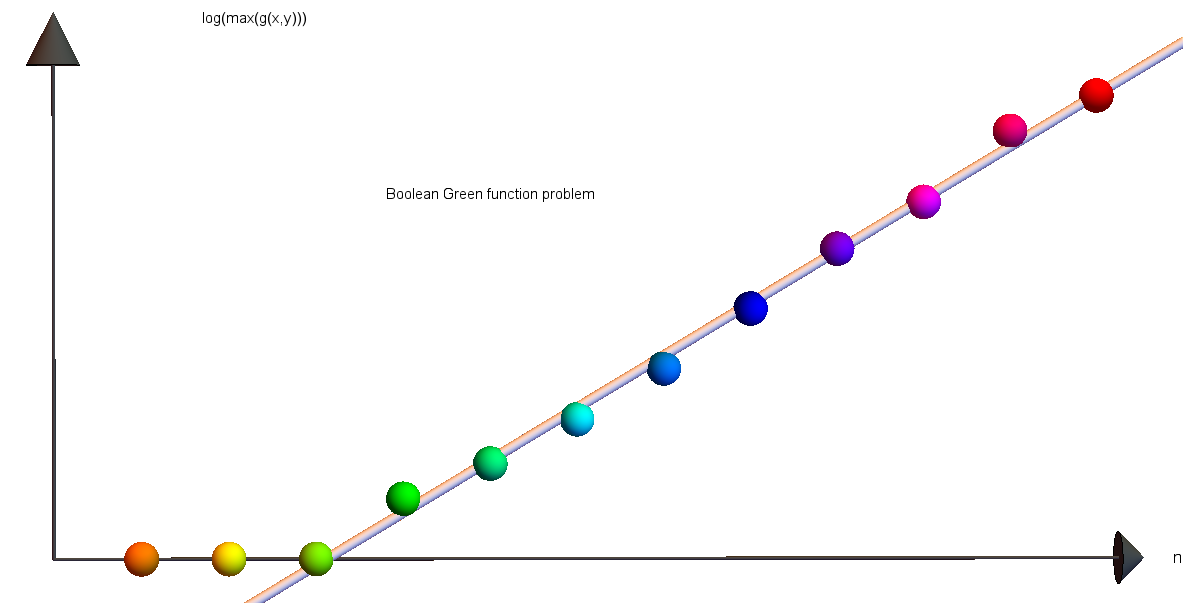
Then there is the question about growth. How fast does this sequence grow?
We can explore this by data fitting. It actually appears as if the growth
is linear on a logarithmic scale indicated exponential growth.
At the beginning at least we see that the maximum max(n) is 2 max(n-1)-1 or
max(n)=2 max(n-1).
max = {1, 1, 1, 2, 3, 5, 9, 18, 36, 62, 141,213}
Fit[Log[max],{1,x,x^2},x]
0.0252498 x^2+0.206081 x-0.498099
|
The determinants
We will talk about determinants in the 4th week.
The
Hadamard maximum determinant problem asks what are the largest possible
determinants in a class of random matrices. In the case of Boolean matrices, this
leads to the sequence
A003432 which is
1, 1, 1, 2, 3, 5, 9, 32, 56, 144, 320, 1458,
Hadamard in 1893 proved that det(A) ≤ sqrt(n^n) if the
entries of A are complex number of length ≤ 1.
For Boolean matrices there is a better upper bound sqrt((n+1)^(n+1))/2^n.
See
this reference.
The sum of the matrix entries
The inverse of a matrix has coefficients g(i,j) which are also known as
Green functions. They have an interpretation as energies. Now, we can
sum them up to get the total energy. Mathematically, what is the sum
of the inverse entries? It appears always to be positive.
We are interested in this also because of previous similar work in
simplicial complexes. See the
energy theorem, where the sum of the Green function matrices is a
topological invariant.
There is an other angle connected with
Counting rooted forests
in a graph and
Cauchy-Binet.
The determinant det(1+L), where L is the Kirchhoff matrix of a graph counts the number
of rooted forests. Chebotarev and Shamis also noted that the Green function entries (1+L)
-1
are probabilities (this follows readily from Cramer). So, the Green function (1+L)
-1 is
always a
doubly stochastic matrix. By the way, I discovered myself the matrix forest theorem as well
as the stochastic property of the Fredholm Matrix 1+L in experiments first, proved it and then found
the Chebotarev-Shamis references from 1997. This is very common in mathematical research. If you do research,
most of the ``discoveries" made turn out already been done. This is only getting more likely as time goes on
as the mathematical knowledge is huge and grows fast. What can be seen in textbooks
is most of the time just the tip of an iceberg. Do we have to worry running out of mathematics? Fortunately
not. In contrary, every discovery triggers three new questions.
Now, also the question of the Green function entries of a random Boolean matrix raised above could
have already been asked and answered. We are currently (Feb 17, 2019), not yet aware of it.
By the way, Chebotarev and Shamis are pictured on
this mathtable
handout from 2016. Here are the pictures of the discoverers of the Matrix Forest Theorem:

|

|
Pavel Chebotarev | Elena Shamis
|
The
matrix forest theorem which counts the number of forests as det(1+L) is even more elegant than the
Cauchy
matrix tree theorem which tells that the number of spanning trees is the pseudo determinant Det(L)
of L. We might mention the pseudo determinant later in the course. The matrix L is always singular but
one can take the product of the non-zero eigenvalues. On the other hand the matrix 1+L is always invertible
because the smallest eigenvalue of 1+L is 1. We will talk about eigenvalues later in the course.
