Data Stories
Starting this fall, there is a
Quantitative Reasoning with Data (QRD)
requirement. This course serves this requirement.
It provides you with a toolkit for thoughtful, critical, and skeptical engagement with
real data sets with the goal to develop a healthy skepticism regarding
data collection and interpretation. The language of multi-variable calculus is
well suited for describing data. Examples: Data are vectors, the dot product
can be interpreted as a covariance, the correlation the cosine of the angle
between vectors. To test sensitivity of data with respect to parameters we need
partial derivatives. Least square fitting is an optimization problem.
For geometric data, probabilities are computed via integration.
These are all topics we study in this course. On this page, we share some `data set stories'
and provide data sets to experiment with.
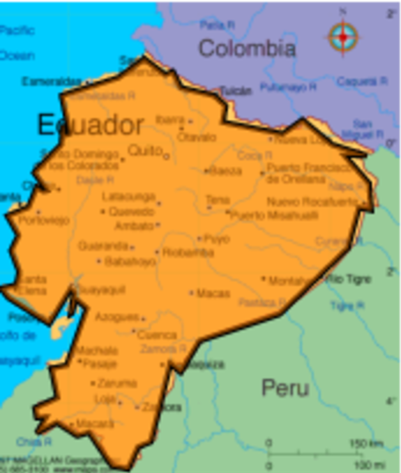
Area of polygons
In the homework for Unit 28
we have a data problem about area of regions. Here is the
Mathematica code which computes the area of a polygon using
Green's theorem:
country = "Ecuador";
CountryData[country, "LandArea"]
A = First[CountryData[country, "SchematicCoordinates"]];
P[{x_, y_}] := 6371*{y*Pi/180, Sin[x*Pi/180]};
B = Map[P, A];
Area[Polygon[B]]
MyArea[A_] := Sum[n = Length[A]; a = A[[k, 1]]; b = A[[k, 2]];
  c = A[[Mod[k, n] + 1, 1]];
  d = A[[Mod[k, n] + 1, 2]]; (a*d - b*c)/2, {k, n}];
MyArea[B]
Here is how you can get a random country:
country = RandomChoice[CountryData[]];
|
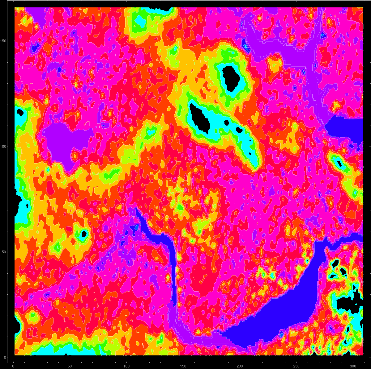
Elevation data
In Homework 16, we have a data project dealing with elevation data.
The code is on the Mathematica page and also
as a Mathematica Notebook.
The picture to the right for example was generated with
A = Reverse[ Normal[GeoElevationData[
     Entity["City", {"Cambridge", "Massachusetts", "UnitedStates"}],
     GeoProjection -> Automatic]]]; ListContourPlot[A]
|
|
We use elevation data from Mathematica. The source are the GIS elevation data.
Here is an
example of the elevation
data near Mt St Helens before and after eruption:
A=Import["http://sites.fas.harvard.edu/~math21a/data/oldhelens.dem","Data"];
B=Import["http://sites.fas.harvard.edu/~math21a/data/newhelens.dem","Data"];
ListContourPlot[A,Contours->20]
ListContourPlot[B,Contours->20]
|
|
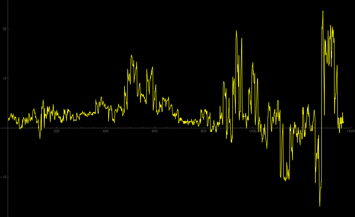
Roller coaster
In this blog,
Robin Deits uses a smartphone to measure the accelerations of a roller coaster
ride on Cedar point, the foremost American roller coaster park.
Robin made the data available on a github repository.
We have the data available on this Mathematica notebook.
|

|
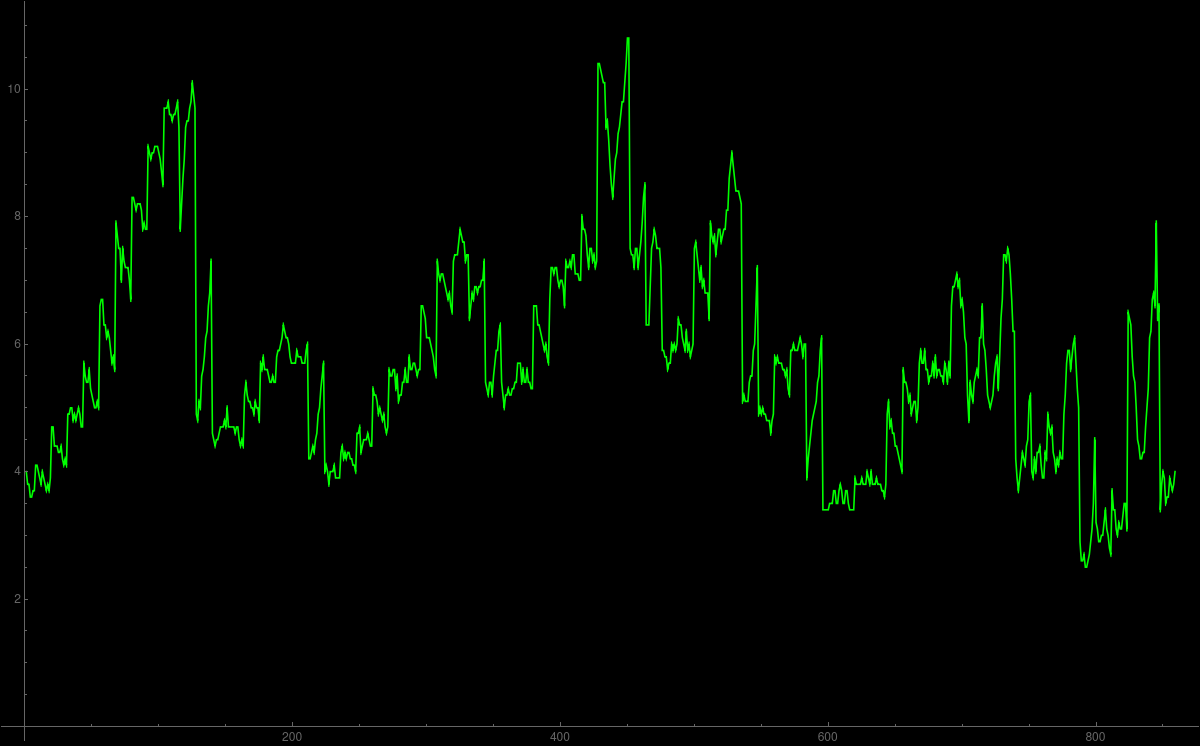
Misery (was mentioned in intro meeting)
The Misery index is the
sum of unemployment and inflation. The term was coined by the economist Arthur Melvin Okun (1928-1980)
in the 1970ies who thought about big questions in economics like equality and efficiency, one of the
big anti-podes also in politics, taxation. It became more complicated with globalization.
Okun created the index in a time, when both quantities were large. It might have influenced elections
like led to the defeat of Richard Ford, where the misery index peaked to 19.9. During the Carter
presidency, it hit 21.98 and might have contributed to Carters defeat in 1980.
Source.
So, here are the latest data sets. There are written so that they can be run directly
in Mathematica. What is important, when curating data is that one always includes the source
so that one can check that the data are correct and not manipulated.
To the right is the outcome of the dataplot.
Of course, the animation in 2D (seen here) is
much cooler.
|
|
Primes ((x-2y+z)2=4 appears in HW 1}
As an experimental number theorist, you investigate prime numbers. Let p(k) denote the k'th
prime number. We have p(1)=2, p(2)=3, p(3)=5, p(4)=7, p(5)=11, etc. We would like to understand
these data. One day, you decide to visualize the primes in space. To do so, you plot the points
(p(k),p(k+1),p(k+2)). Here are the data points obtained with
Table[{Prime[k],Prime[k+1],Prime[k+2]},{k,8}]
When looking at the points we notice that x-2y+z is often either 2 or -2. The quantity x-2y+z
measures some kind of acceleration. While v(k) = p(k+1)-p(k) is a rate of change, the rate of change
of the rate of change is v(k+1)-v(k) = [p(k+2)-p(k+1)] - [p(k+1)-p(k)] = p(k+2)-2p(k+1)+p(k).
From the first 8 data points 75 percent have |x-2y+z|=2. To experiment more, use the computer
f[n_]:=Sum[If[(Prime[k]-2Prime[k+1]+Prime[k+2])^2==4,1,0],{k,n}]/n;
From the first 100 data points 45 are on the set S = { (x-2y+z)2=4 }
The function f(n) gives the fraction of points X(k) which are on S if
k runs from 1 to n, divided by n. For example, f(8)=6/8 or f(100)=45/100.
An unsolved problem is to decide how f(n) behaves for large n. Does it
go to zero? If yes, how fast? Nobody seems to have looked at it yet. This example shows that
data also can appear in purely mathematical frame works. Almost all theorems in mathematics,
almost all conjectures come from experimenting with data at first. In the case of primes, one has
first noticed that there appear to be infinitely many, then proved it. Gauss, without a
computer of course, looked at the prime data and conjectured how the number of primes grow. This
was later proven and is called the prime number theorem.
For differences of primes, one believes (again, by looking at data) that there are
infinitely many cases, where (x,y) = (p(k),p(k+1)) are on the line y-x=2. This is the famous
open prime twin conjecture.
|
x    y    z           x-2y+z
----------------------------
2    3    5               1
3    5    7               0
5    7    11              2
7    11   13             -2
11   13   17              2
13   17   19             -2
17   19   23              2
19   23   29              2

We see that a spacial representation of data leads to new questions and
possibly insight. In this case the problem is a pure mathematical problem about
prime numbers. Prime numbers used to be a domain which was of interest only for
theoretical mathematicians. Because of cryptological applications, it has become one of
the most applied topics of mathematics overall.
|
University ranking
(* https://www.topuniversities.com/university-rankings/world-university-rankings/2019 *)
(* Uni, Overall, Academic, Employer, Fac/Stu,cite,intern faculty, intern. students *)
A={
{"MIT" ,100 ,100 ,100 ,100 ,99.8,100 ,95.5},
{"Stanford" ,98.6 ,100 ,100 ,100 ,99 ,99.8 ,70.5},
{"Harvard" ,98.5, 100 ,100 ,99.3,99.8,92.1 ,75.7},
{"Caltech" ,97.2, 98.7,81.2,100 ,100 ,96.8 ,90.3},
{"Oxford" ,96.8, 100 , 100,100 , 83 ,99.6 ,98.8},
{"Cambridge" ,95.6, 100 , 100,100 ,77.2,99.4 ,97.9},
{"ETH" ,95.3, 98.2,96.2,82.4,98.7, 100 ,98.6},
{"Imperial" ,93.3, 98.7,99.9,99.9,67.8, 100 , 100},
{"Chicago" ,93.2, 99.6,90.7,97.4,83.6,74.2 ,82.5},
{"UCL" ,92.9, 99.3,99.2,99.2,66.2,98.7 , 100}
};
Capital, Labor and Production values
The original article of Cobb and Douglas
A Theory of Production, American Economic Review, 18/1, 1928 contains the following data:
(* Year,Capital,Labor,Production   *)

A={
{1899,100,100,100},
{1900,107,105,101},
{1901,114,110,112},
{1902,122,118,122},
{1903,131,123,124},
{1904,138,116,122},
{1905,149,125,143},
{1906,163,133,152},
{1907,176,138,151},
{1908,185,121,126},
{1909,198,140,155},
{1910,208,144,159},
{1911,216,145,153},
{1912,226,152,177},
{1913,236,154,184},
{1914,244,149,169},
{1915,266,154,189},
{1916,298,182,225},
{1917,335,196,227},
{1918,366,200,223},
{1919,387,193,218},
{1920,407,193,231},
{1921,417,147,179},
{1922,431,161,240}
};