Updates on the Valuation paper
Here are some updates (mini blog) on Gauss-Bonnet for multi-linear valuations [ArXiv], On the local version, where minor updates are done. Also: A handout to a mathtable talk and a case analysis [PDF] showing how to distinguish the cylinder from the Moebius strip cohomologically.- [April 6, 2016] Intersection cohomology is formally related to the tensor product of the singular chain complexes which has an exterior derivative d(a ⊗ b) = da ⊗ b + (-1)deg(a) a ⊗ b. But there is an essential difference as we don't look really at the tensor product of the chain complexes, which is what we get if we when taking the chain complex of the graph product of the graph with itself. In interaction cohomology we only evaluate the function on the interacting parts. Without that we would just get a cohomology equivalent to simplicial cohomology of the product (this is the discrete de Rham statement). It is difficult to see how that would look classically look similar than intersection cohomology since for a manifold M, where we evaluate F(x,y) at two different points. In some sense, we only look at functions on pairs of points which are infinitesimally close.
- [April 3, 2016] In the Euler characteristic case, we also computed the Lefschetz zeta function exp( sum chi(Tn),G) zn/n) as custom in a Lefschetz context. Here chi(T,G) is the Lefschetz number of T, the super trace of UT on simplicial cohomology. In the case of the identity automorphism T, it is exp(chi(T) sum zn/n) = [exp( sum zn/n)]chi(G) = (1-z)-chi(G) confirming that the order of the pole z=1 is an interesting quantity. The situation is identical for the Wu characteristic, their cohomology and Lefschetz number. Also, in the same way than the zeta function can be written as a Ruelle zeta function involving periodic points of T (as done in the fixed point paper), this is also the case in the Wu characteristic case. (The proof in that follows almost verbatim the proof of Ruells book. I had been lucky to be a student of a Nachdeplomvorlesung (graduate course) taught by Ruelle on dynamical zeta functions at ETH). As in the Euler characteristic case, one can also take the product of these zeta functions over the automorphism group to get a zeta function which now only depends on geometry. Like spectral properties of a graph, these zeta functions depend on the symmetry. But what is nice is that since also the Wu characteristic or the Lefschetz numbers belonging to intersection cohomology are invariant under Barycentric refinement, these numbers are combinatorial invariants which therefore must play a role in the continuum. Now, automorphisms are rather confining. It corresponds to an isometry in the continuum limit. For a finite simple graph, the situation seems not so exciting from a dynamical systems point of view as all orbits are periodic. This is not the case. Nonstandard analysis has shown that one can do all topology on compact sets on finite sets. Ed Nelson has formulated all continuum stochastic process theory nicely on finite sets (radically elementary probability theory). As Nelson has shown, it is merely a matter of language (extend ZFC using three axioms NST telling what "standard" means is enough). As a student, I once presented in a Specker seminar a proof of the Fuerstenberg multiple recurrence theorem in the internal set theory language of nonstandard analysis. Fuerstenberg had used his multiple-recurrence theorem for commuting actions to prove the van der Waerden theorem, a purely combinatorial result on the existence of arbitrary long arithmetic sequences in one of the partitions of the integers into finitely many sets. The reason why things are simple in a nonstandard analysis setup is that the periodicity of an orbit (with nonstandard period) corresponds to a recurrent point (and actual periodic orbits with standard minimal period). For a Z action on a compact space, the existence of recurrence becomes a triviality (for Zd actions, there is still work to do). Similarly, as most of school calculus collapses as Nelson has illustrated in countless places. For example, Bolzano's theorem: to see that a continuous function takes its maximum on a compact set, just look at the maximum on the finite set F representing the compact set X (F is a finite set such that every point in is infinitesimally close to a point in F. Two points x,y are infinitesimally close if their distance d(x,y) is smaller than any standard positive real number.) The genius of Nelsons version of nonstandard analysis was that all mathematics we know built from ZFC is included. There is a theorem then which proves that if ZFC is consistent, then ZFC + NST is consistent. The three additional axioms tell how to deal with the new concept "standard". No ultra filter stuff like in Robinson's approach is needed.
- [April 2, 2016] A question which starts to nag is whether the
quadratic interaction cohomology H*(G) satisfies the Eilenberg-Steenrod
axioms, when generalized to the relative case H*(G,A).
In order to make sense of the question, there is a need to specify
what is understood by "topology" or "homotopy" as both notions are needed.
The quadratic interaction cohomology H*(G) is defined
for finite simple graphs or simplicial compelexes.
Classical notions of topology or homotopy do not work without digressing
to geometric realizations in Euclidean space which we do not want to do
[as it would not only be betrayal to combinatorics but also not be healthy
from the computer science point of view which anyway needs finite structures].
A reasonable finite classical point set
topology on a finite graph is the discrete topology as it should be related to
the natural notion of geodesic distance on the graph. Any finite graph equipped with
a geodesic distance generates the discrete topology because 1-point-sets {v} are
both open and closed. A suggestion to render graphs into a category of topological
spaces was suggested here
(not submitted yet to any journal).
So far, the suggestion looks good: it allows to treat graphs
as higher-dimensional objects and emancipate them from the usual restriction to be a
1-dimensional a simplicial complex, a jacket which has been imposed on graph theory.
The Čech covering approach allows to deal with graphs in a "rubber geometry"
type manner and for example render the octahedron homeomorphic to the
icosahedron or see that in full generality,
the Barycentric refinement of a graph G is homeomorphic to G. It also agrees with the classical
notion of homeomorphism if the graph has no triangles.
(The Barycentric refinement is not the classical notion considered in
combinatorial graph theory, where only edges are refined but
defined as the product G x K1. )
In the proposed notion, the two notions
'homotopy' and "dimension' combine to define what a continuous map or homeomorphism is in
a purely discrete setting.
Graphs with such a topology form again a category but the same graph can
represent different objects and different topologies on the same set produce
different objects or different objects topology become equivalent.
[Why use the language of graph theory? First, graphs are intuitive. Second, there is no ambiguity
as the everybody agrees what the category of finite simple graphs is.
And thirdly, computer algebra systems use graph theory built into their language already.]
Homotopy notions allow deformations, dimension notions make sure that these deformations are not too broad. We can't have for example the cylinder to be homeomorphic to a circle. Fortunately, a notion of homotopy for discrete objects has been defined already by A.N. Whitehead and adapted to graphs by A.V. Ivashchenko [in the 90ies (then at MIT) who is like R. Forman one of the pioneers of translating notions from the continuum to the discrete] and simplified in a paper of Chen-Yau-Yeh: define a graph to be collapsible if it is either the 1-point graph K1 or if there exists a vertex such that its unit sphere is collapsible. Taking away such a vertex together with all connections produces a smaller graph. The reverse construction is to take a contractible subgraph and build a cone over it to get a larger graph. Combining such elementary collapse or expansion steps leads to the notion of homotopy and so produces equivalence classes in the category of finite simple graphs. A graph which is homotopic to a point is called contractible (≠ contractible, as the "dunce hat" indicates). In the continuum, there is also a notion of homotopy for subsets of a given host topology. This is used for the definition of homotopy groups. For example, a closed path in the 2-dimensional plane is homotopic to a point as it can be "pulled together" to a point. As a space itself, the closed path is not homotopic to a point as its cohomology is different. One looks at continuous maps from X to X and considers two such maps f0,f1 homotopic if there exists a continuous map F from X x [0,1] to Y such that F(x,0)=f0 and F(x,1)=f1. The curve deformation is a homotopy of parametrizations of continuous maps from the circle to the space. When translating such a notion to the discrete, it requires not only a notion of "continuity" meaning topology but also a notion of "Cartesian product". That is why I searched last year systematically for a product which can be used in graph theory (the usual notions in graph theory are all inadequate) and wrote this (also not yet submitted). By having a product and notion of continuity, the classical definition of homotopy can be used but without any referral to the continuum. A closed curve in a graph for example is a continuous map from a discrete circle Cn (with n>3) to a graph G and a "simple closed curve" is a map, where the image is homeomorphic in the new sense. As the notion of homeomorphism and product is compatible with Barycentric subdivision, this is natural and in sense of standard notions in the continuum: (I mean this in the sense of working with finite computer implementations of continuum objects). Lets come back to the notion of Eilenberg-Steenrod axioms which require to extend the notion to a relative quadratic cohomology H((G1,A1),(G2,A2)), where A1 is a subgraph of G1 and A2 is a subgraph of G2. Lets briefly glance at the axioms:
[For simplicity, we restrict to G1 = G2 (the Wu characteristic case, rather than the more general Wu interaction case H(G1,G2) involving pairs (x,y) with x in G1 and y in G2. This is also to avoid the notational potential confusion that H*(G,A) denotes the relative cohomology rather than what we have used for interaction cohomology H(G1,G2) before.] - Excision: To make the inclusion (G-U,A-U) -> (X,A) induce an isomorphism of cohomology, it appears necessary that the subgraph U entering there is in the interior of A in the sense that also the unit ball of U within G is a subgraph of A. (This has to be specified what interior means as we don't have a classical point set topology but a topology together with a sub-basis, a setup closer to point-less topology or Cech or sheaf constructions.)
- Homotopy:
Homotopic graphs do not have the
same interaction cohomology, as growing a hair on a circle or enlarging K1 to K2
shows already. But what is not yet excluded is what enters in Eilenberg-Steenrod:
if f,g: (G,A) -> (H,B) are homotopic (using the notion of
continuity and graph product just mentioned), then the corresponding linear maps
on cohomology be the same. More generally, in the interaction case,
homotopic maps f,g: ((G1,A1),(G2,A2)) -> ((H1,B1),(H2,B2)) should induce the
same maps on cohomology.
Evenso, we don't like to go into the continuum, a reason for this could be invariance under
Barycentric subdivision so that there is a continuum limiting case for which the homotopy
deformation invariance can be seen.
[Related: Even so only few experiments have been done, they indicate that if B is homotopic to A within the interior of G, then the cohomology H(G,A) and H(G,B) are the same even if the individual cohomologies H(A,A) and H(B,B) of the subgraphs can be different. For example, if A = K1 and B=K2 both in the interior of G, then H*(G,A)=H*(G,B)). But if A = K1 and B is a sphere, then H(G,A) and H(G,B) disagree. The reason for the agreement could be that as in the case of a point, there might be a general formula relating the interaction cohomology H(G,A) of a subgraph A in the interior of G with the simplicial cohomology of the sphere S(A) (which is the graph generated by all vertices in G in distance 1 from A), a formula verified in the case, when A is a one point graph. Now, since, simplicial cohomology is invariant under homotopy, this could do the job.] - Dimension: the dimension axiom holds because a one-point graph G=K1 has trivial interaction cohomology Hn(G) for all n>0. So, it is an ordinary cohomology, provided the other axioms hold.
- Additivity: The additivity axiom is clear from the definitions: taking two disjoint graphs adds up the cohomologies. This is no different than in simplicial cohomology.
- Exactness: We believe the exactness axiom to hold. It would be a surprise to fail since interaction cohomology is formally so close to simplicial cohomology.
| dim(Hp(v,G)) = dim(Hp-1(S(v))) |
| w(v,G) = 1-X(S(v)) |
- Hp(A,G) = Hp(A,B(A)) where B(A) is a neighborhood of radius 1 of A. For example, if A is a one point graph (a case we will look at first, then Hp(A,G) = Hp(p,B(p)) only depends on the unit ball of p.
- The cohomology satisfies Kuenneth and w(A,G) is compatible with the product w(A x B,G x H) = w(A,G) w(G,H). Especially, w(A,G) is invariant under simultaneous Barycentric subdivisions.
- The fact that we have invariance under Barycentric subdivision will imply that Hp(A,G) is topological in the sense that if A is deformed nicely within G by analogues of homeomorphisms while fixing G, then the cohomology does not change. This is a homotopy invariance.
- If p is a vertex in G with positive vertex degree then H0(p,G)=0.
- If p is a vertex in G with zero vertex degree, then H0(p,G) = 1.
- If p is not contained in a triangle then H1(p,G) = deg(p)-1
- If the unit sphere S(p) has k connected components, then H1(p,G) = k-1.
Proof of 2: if the vertex p is isolated, then there are no vertex-edge pairs and d0f=0 for any f. Since the set of 0-forms is just one dimensional as there is only one 0-0 vertex interaction which involves p, the cohomology is one dimensional.
Proof of 3: we need to understand the vector space H1(p,G) = ker(d1)/im(d0) if e1,...,ek are the edges connected to the vertex p, then the kernel of d1 (the vector space of closed forms) is k dimensional since there are no edge-edge nor point triangle interactions by assumption. The image of d0 consists of functions on vertex-edge pairs (p,(pb)) given by df(p,(pb)) = f(p,p) showing that exact 1-forms are all locally constant f(p,(pb))=c The quotient can be seen as the set of all functions on neibhboring edges of p, for which the sum of the function values is zero. This vector space is k-1= deg(p)-1 dimensional.
Proof of 4: Its very similar than before but now, the presence of the triangle shows there are much less closed forms as there are edge-edge interactions in 2forms which come as boundaries of the triangle. Let (pq) and (pr) be two edges bounding a triangle t =(pqr), then df(p,(pqr)) = f(p,qr)-f(p,pr)+f(p,pq). Since p and qr do not interact, this is -f(p,pr)+f(p,pq) =0. This means that the function values must agree on edges which share a common triangle.
If A is a subgraph with maximal dimension k of and G has maximal dimension d, then there are k+d+1 cohomologies H^*(A,G) which can be studied. We have just seen that the number of connected components in the unit sphere of a vertex has a cohomological interpretation. In a graph without triangles this is the vertex degree.
The second case is if G is a bundle with base A. Like if G is the product of A with an other graph (which is a trivial bundle). In this case we always measured so far that Hp(A,G)=0 for all p. And this seems to hold also for nontrivial bundles like the Moebius strip and A is a circle. Only if A is thickened, we believe to get interesting interaction cohomologies.
|
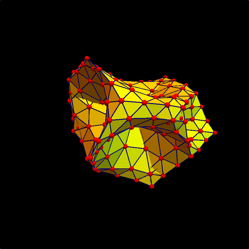
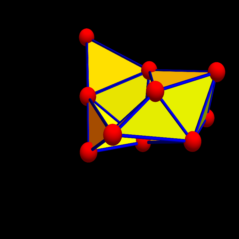
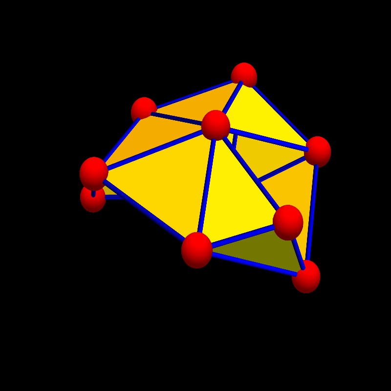
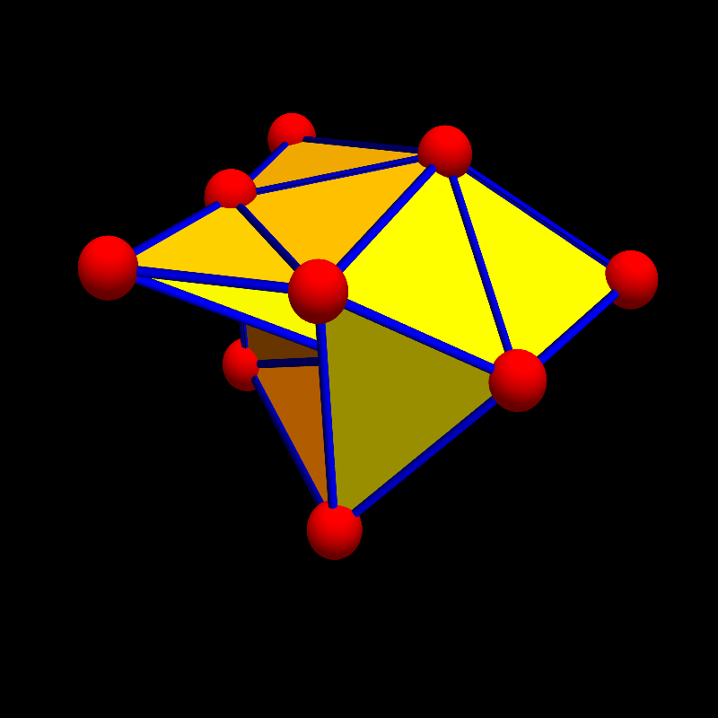
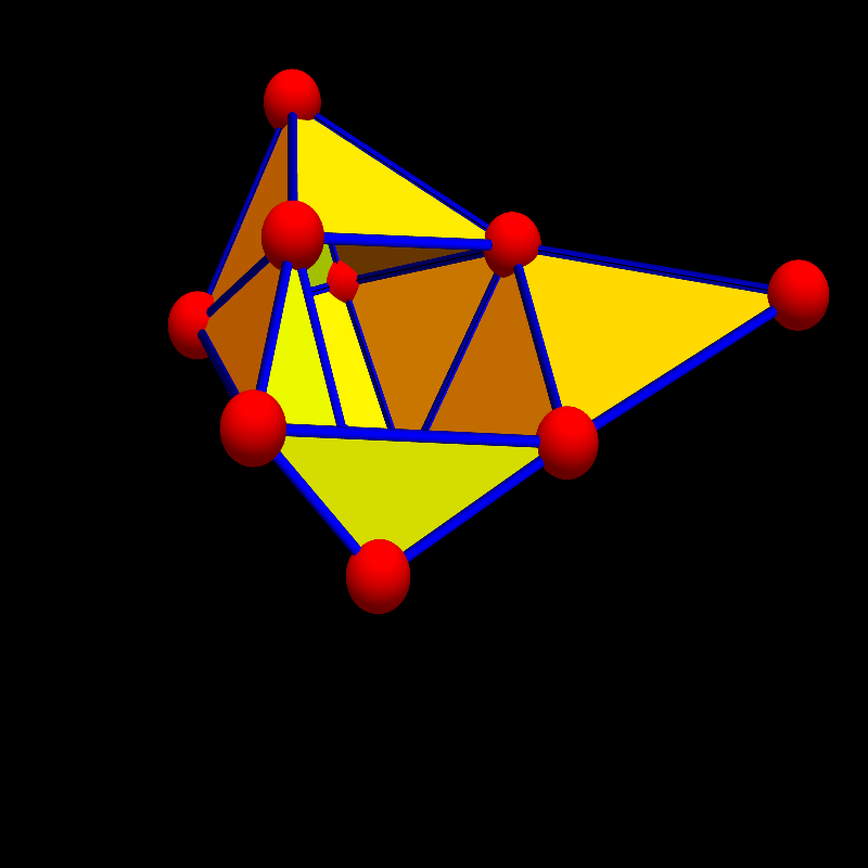
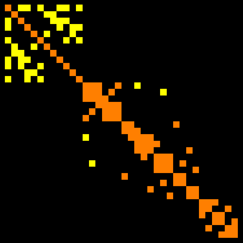
[March 20, 2016] When looking through the computations below, an other remarkable
example is the Dunce hat,
a prototype of a contractible but not collapsible space. It was introduced in 1963 by Zeeman
in the context of the Poincaré conjecture.
As it is contractible (homotopic to a point), its cohomology is trivial. Of course
we can compute and investigate the geometry more conveniently using graphs.
The picture shows a twice Barycentric refined version of this graph
(using a tamed refinement method which does not grow the vertex degrees). This does not
change the failure to collapse as the graph first needs to be thickend and become a
three dimensional object temporarily before being able to shrink it a point.
The Betti vector of the graph is (1,0,0)
which is the same than the Betti vector of the 2-disc (i.e. Wheel graphs). But now,
the interaction cohomology Betti vector is (0, 0, 0, 1, 2), showing that it is not
homeomorphic to a disc. All discs have the interaction cohomology Betti vector (0,0,1,0,0).
Both have Wu characteristic 1. Again, neither simplicial cohomology, nor
Wu characteristic distinguish the dunce hat from the disc. But interaction cohomology
does. (Side remark: The cubic interaction cohomology is not yet computed due to too much complexity. The graph we use has f-vector 17, 52, 36 and 62769 cubic interactions. The size of the cubic interaction Laplacian, a 62769 x 62769 matrix which is too large. We could imagine that this could be implementable fast in a specialized C program, where the programming language allows to work on much larger data structures without loading therm first in full to memory like Mathematica does with matrices. Computing the kernel of a matrix only needs row reduction, which allows to work on the matrix locally without seeing the entire object. ) |
 |
 |
 |
 |
 | Interaction cohomology seems indeed be able to distinguish between the cylinder and the Moebius strip as the quadratic interaction cohomologies H2 and H3 are both different. Stiefel-Whitney classes can do that too, but these are invariants for vector bundles. The interaction cohomology tool does not need a bundle structure. It works for any graphs. While not interesting for manifolds, where one can derive the quadratic cohomology from simplicial cohomology, it could be useful for varieties. |

|
 | Here are two graphs with the same f-vector, the same simplicial cohomology, the same quadratic and cubic Wu characteristic, but for which the quadratic cohomology distinguishes it. |
 |
 | Here is a better example: for these two graphs, the f-vector (9, 18, 9, 1) and f-matrix {{{9, 36, 27, 4}, {36, 136, 96, 13}, {27, 96, 65, 8}, {4, 13, 8, 1}} are both the same. The Betti vector is the same (1, 2, 0, 0) so linear simplicial cohomology is the same but the quadratic Wu cohomology differs: It is {0, 0, 6, 3, 0, 0, 0} for the first graph and {0, 0, 4, 1, 0, 0, 0} for the second graph. |
 |
| The second interaction cohomology of the Moebius strip G is completely zero: the second Dirac operator D and Laplacian L=D2 are invertible. Since the interaction cohomology of G does not agree with the interaction cohomology of the cylinder, topological realizations of the two simplicial complexes can not be homeomorphic. We have so obtained a simple classical algebraic tool to distinguish the two graphs: just compute some incidence matrices and determine their nullity. The interaction Betti numbers allow to distinguish graphs which usual cohomology can not. |
|
Euler chi  Betti(1)   Wu(2)   Betti(2)    Wu(3)   Betti(3)
--------------------------------------------------------------------------
0          (1,1,0)    0       (0,0,0,0,0)  0      (0,0,0,0,1,1,0)       Moebius
0          (1,1,0)    0       (0,0,1,1,0)  0      (0,0,0,0,1,1,0)       Cylinder
Both simplicial cohomology as well as cubic interaction cohomology does not "See" the diffference between the two graphs. The quadratic interaction cohomology does.
To make sure that there is not some stupid mistake, lets give more details. The Moebius strip is defined as a finite simple graph G with vertex set {1,2,3,4,5,6,7,8} and edges set E:
UndirectedGraph[Graph[
{1 -> 2, 1 -> 5, 1 -> 8, 2 -> 3, 2 -> 5, 2 -> 6, 3 -> 4, 3 -> 6,
 3 -> 7, 4 -> 5, 4 -> 7, 4 -> 8, 5 -> 6, 5 -> 8, 6 -> 7, 7 -> 8}]]
The Whitney complex of the graph G is here:
{1}, {2}, {3}, {4}, {5}, {6}, {7}, {8}           (Vertices)
{1, 2}, {1, 5}, {1, 8}, {2, 3}, {2, 5},
{2, 6}, {3, 4}, {3, 6}, {3, 7}, {4, 5},          (Edges)
{4, 7}, {4, 8}, {5, 6}, {5, 8}, {6, 7}, {7, 8}}
{1, 2, 5}, {1, 5, 8}, {2, 3, 6}, {2, 5, 6},
{3, 4, 7}, {3, 6, 7}, {4, 5, 8}, {4, 7, 8},      (triangles)
Here is the Wu interaction complex given by all the 424 ordered pairs of
simplices in G which intersect. One can get the number 424 also by adding up all numbers
in the f-matrix of the Moebius graph G. This f-matrix is
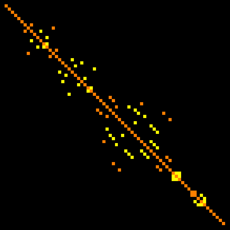
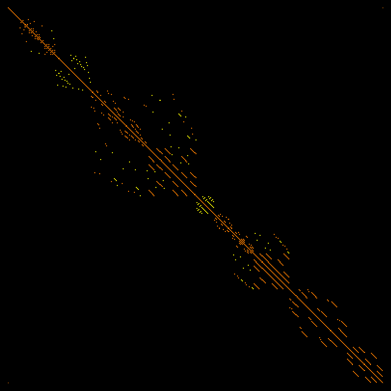
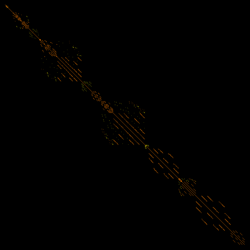
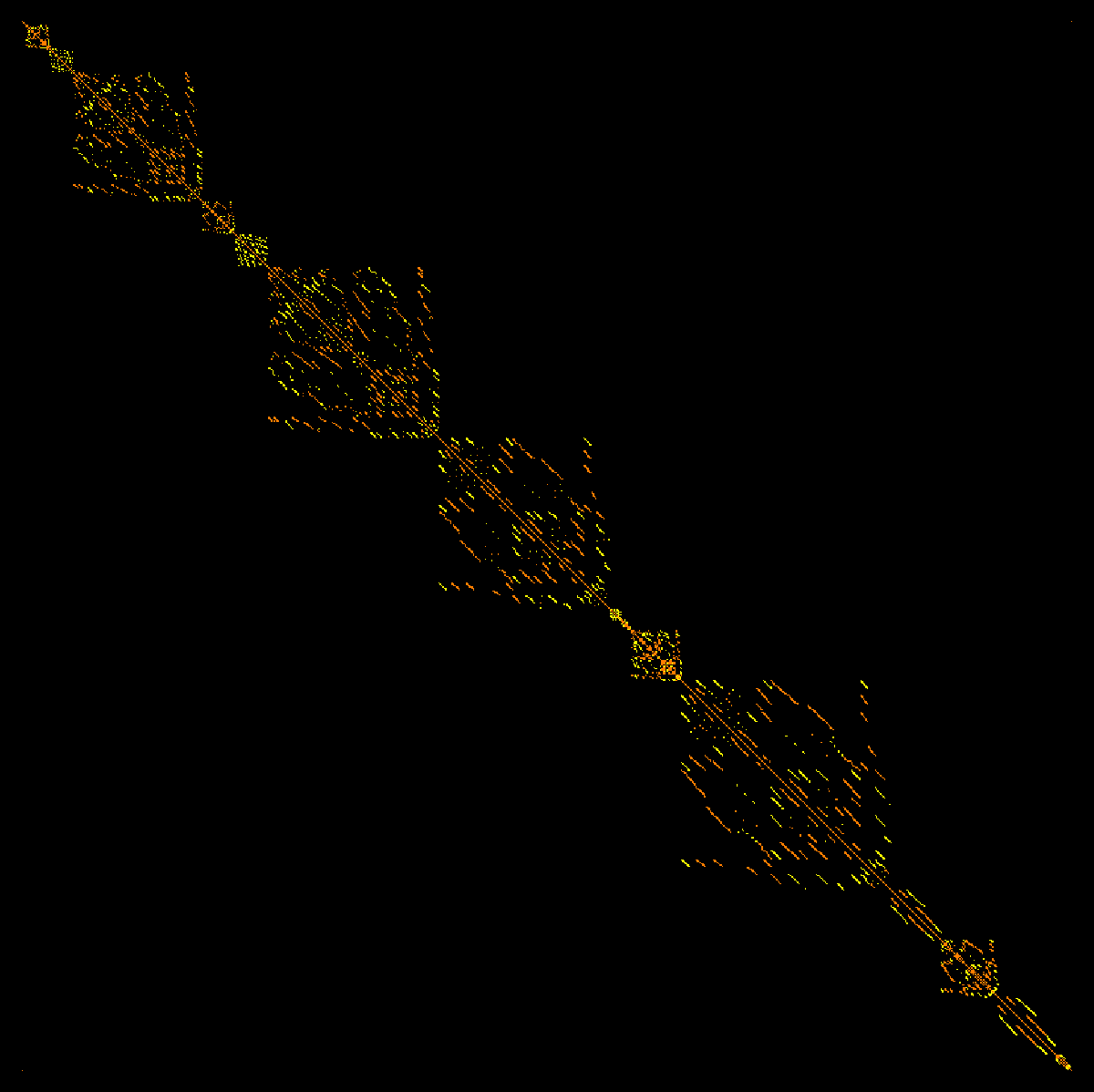
 8     32    24
32    114    74
24     74    42
The Dirac operator D and the Laplacian L=D2 of G are both 424x424 matrices. A picture of the Laplacian is given below. But first to the quadratic interaction complex, defined by all the interacting pairs of simplices in the graph:
(* First the 8 vertex-vertex interactions, these are the 0-forms  *)
{{8}, {8}}, {{7}, {7}}, {{6}, {6}}, {{5}, {5}}, {{4}, {4}},
{{3}, {3}}, {{2}, {2}}, {{1}, {1}},

(* Now the 32+32 vertex-edge interactions. These are the 1-forms  *)
{{7, 8}, {8}}, {{7, 8}, {7}}, {{6, 7}, {7}}, {{6, 7}, {6}},
{{5, 8}, {8}}, {{5, 8}, {5}}, {{5, 6}, {6}}, {{5, 6}, {5}},
{{4, 8}, {8}}, {{4, 8}, {4}}, {{4, 7}, {7}}, {{4, 7}, {4}},
{{4, 5}, {5}}, {{4, 5}, {4}}, {{3, 7}, {7}}, {{3, 7}, {3}},
{{3, 6}, {6}}, {{3, 6}, {3}}, {{3, 4}, {4}}, {{3, 4}, {3}},
{{2, 6}, {6}}, {{2, 6}, {2}}, {{2, 5}, {5}}, {{2, 5}, {2}},
{{2, 3}, {3}}, {{2, 3}, {2}}, {{1, 8}, {8}}, {{1, 8}, {1}},
{{1, 5}, {5}}, {{1, 5}, {1}}, {{1, 2}, {2}}, {{1, 2}, {1}},
{{8}, {7, 8}}, {{8}, {5, 8}}, {{8}, {4, 8}}, {{8}, {1, 8}},
{{7}, {7, 8}}, {{7}, {6, 7}}, {{7}, {4, 7}}, {{7}, {3, 7}},
{{6}, {6, 7}}, {{6}, {5, 6}}, {{6}, {3, 6}}, {{6}, {2, 6}},
{{5}, {5, 8}}, {{5}, {5, 6}}, {{5}, {4, 5}}, {{5}, {2, 5}},
{{5}, {1, 5}}, {{4}, {4, 8}}, {{4}, {4, 7}}, {{4}, {4, 5}},
{{4}, {3, 4}}, {{3}, {3, 7}}, {{3}, {3, 6}}, {{3}, {3, 4}},
{{3}, {2, 3}}, {{2}, {2, 6}}, {{2}, {2, 5}}, {{2}, {2, 3}},
{{2}, {1, 2}}, {{1}, {1, 8}}, {{1}, {1, 5}}, {{1}, {1, 2}},

(* And now to the 16 edge-edge self interactions. These are 2-forms*)
{{7, 8}, {7, 8}}, {{7, 8}, {6, 7}}, {{7, 8}, {5, 8}}, {{7, 8}, {4, 8}},
{{7, 8}, {4, 7}}, {{7, 8}, {3, 7}}, {{7, 8}, {1, 8}}, {{6, 7}, {7, 8}},
{{6, 7}, {6, 7}}, {{6, 7}, {5, 6}}, {{6, 7}, {4, 7}}, {{6, 7}, {3, 7}},
{{6, 7}, {3, 6}}, {{6, 7}, {2, 6}}, {{5, 8}, {7, 8}}, {{5, 8}, {5, 8}},

(* And now the 98 edge-edge interactions  Also this are 2 forms    *)
{{5, 8}, {5, 6}}, {{5, 8}, {4, 8}}, {{5, 8}, {4, 5}}, {{5, 8}, {2, 5}},
{{5, 8}, {1, 8}}, {{5, 8}, {1, 5}}, {{5, 6}, {6, 7}}, {{5, 6}, {5, 8}},
{{5, 6}, {5, 6}}, {{5, 6}, {4, 5}}, {{5, 6}, {3, 6}}, {{5, 6}, {2, 6}},
{{5, 6}, {2, 5}}, {{5, 6}, {1, 5}}, {{4, 8}, {7, 8}}, {{4, 8}, {5, 8}},
{{4, 8}, {4, 8}}, {{4, 8}, {4, 7}}, {{4, 8}, {4, 5}}, {{4, 8}, {3, 4}},
{{4, 8}, {1, 8}}, {{4, 7}, {7, 8}}, {{4, 7}, {6, 7}}, {{4, 7}, {4, 8}},
{{4, 7}, {4, 7}}, {{4, 7}, {4, 5}}, {{4, 7}, {3, 7}}, {{4, 7}, {3, 4}},
{{4, 5}, {5, 8}}, {{4, 5}, {5, 6}}, {{4, 5}, {4, 8}}, {{4, 5}, {4, 7}},
{{4, 5}, {4, 5}}, {{4, 5}, {3, 4}}, {{4, 5}, {2, 5}}, {{4, 5}, {1, 5}},
{{3, 7}, {7, 8}}, {{3, 7}, {6, 7}}, {{3, 7}, {4, 7}}, {{3, 7}, {3, 7}},
{{3, 7}, {3, 6}}, {{3, 7}, {3, 4}}, {{3, 7}, {2, 3}}, {{3, 6}, {6, 7}},
{{3, 6}, {5, 6}}, {{3, 6}, {3, 7}}, {{3, 6}, {3, 6}}, {{3, 6}, {3, 4}},
{{3, 6}, {2, 6}}, {{3, 6}, {2, 3}}, {{3, 4}, {4, 8}}, {{3, 4}, {4, 7}},
{{3, 4}, {4, 5}}, {{3, 4}, {3, 7}}, {{3, 4}, {3, 6}}, {{3, 4}, {3, 4}},
{{3, 4}, {2, 3}}, {{2, 6}, {6, 7}}, {{2, 6}, {5, 6}}, {{2, 6}, {3, 6}},
{{2, 6}, {2, 6}}, {{2, 6}, {2, 5}}, {{2, 6}, {2, 3}}, {{2, 6}, {1, 2}},
{{2, 5}, {5, 8}}, {{2, 5}, {5, 6}}, {{2, 5}, {4, 5}}, {{2, 5}, {2, 6}},
{{2, 5}, {2, 5}}, {{2, 5}, {2, 3}}, {{2, 5}, {1, 5}}, {{2, 5}, {1, 2}},
{{2, 3}, {3, 7}}, {{2, 3}, {3, 6}}, {{2, 3}, {3, 4}}, {{2, 3}, {2, 6}},
{{2, 3}, {2, 5}}, {{2, 3}, {2, 3}}, {{2, 3}, {1, 2}}, {{1, 8}, {7, 8}},
{{1, 8}, {5, 8}}, {{1, 8}, {4, 8}}, {{1, 8}, {1, 8}}, {{1, 8}, {1, 5}},
{{1, 8}, {1, 2}}, {{1, 5}, {5, 8}}, {{1, 5}, {5, 6}}, {{1, 5}, {4, 5}},
{{1, 5}, {2, 5}}, {{1, 5}, {1, 8}}, {{1, 5}, {1, 5}}, {{1, 5}, {1, 2}},
{{1, 2}, {2, 6}}, {{1, 2}, {2, 5}}, {{1, 2}, {2, 3}}, {{1, 2}, {1, 8}},
{{1, 2}, {1, 5}}, {{1, 2}, {1, 2}},

(* And now 24+24 the vertex-triangle interactions, 2-forms too       *)
{{4, 7, 8}, {8}}, {{4, 7, 8}, {7}}, {{4, 7, 8}, {4}}, {{4, 5, 8}, {8}},
{{4, 5, 8}, {5}}, {{4, 5, 8}, {4}}, {{3, 6, 7}, {7}}, {{3, 6, 7}, {6}},
{{3, 6, 7}, {3}}, {{3, 4, 7}, {7}}, {{3, 4, 7}, {4}}, {{3, 4, 7}, {3}},
{{2, 5, 6}, {6}}, {{2, 5, 6}, {5}}, {{2, 5, 6}, {2}}, {{2, 3, 6}, {6}},
{{2, 3, 6}, {3}}, {{2, 3, 6}, {2}}, {{1, 5, 8}, {8}}, {{1, 5, 8}, {5}},
{{1, 5, 8}, {1}}, {{1, 2, 5}, {5}}, {{1, 2, 5}, {2}}, {{1, 2, 5}, {1}},
{{8}, {4, 7, 8}}, {{8}, {4, 5, 8}}, {{8}, {1, 5, 8}}, {{7}, {4, 7, 8}},
{{7}, {3, 6, 7}}, {{7}, {3, 4, 7}}, {{6}, {3, 6, 7}}, {{6}, {2, 5, 6}},
{{6}, {2, 3, 6}}, {{5}, {4, 5, 8}}, {{5}, {2, 5, 6}}, {{5}, {1, 5, 8}},
{{5}, {1, 2, 5}}, {{4}, {4, 7, 8}}, {{4}, {4, 5, 8}}, {{4}, {3, 4, 7}},
{{3}, {3, 6, 7}}, {{3}, {3, 4, 7}}, {{3}, {2, 3, 6}}, {{2}, {2, 5, 6}},
{{2}, {2, 3, 6}}, {{2}, {1, 2, 5}}, {{1}, {1, 5, 8}}, {{1}, {1, 2, 5}},

(* And now the 74+74 edge-triangle interactions  3 forms              *)
{{7, 8}, {4, 7, 8}}, {{7, 8}, {4, 5, 8}}, {{7, 8}, {3, 6, 7}},
{{7, 8}, {3, 4, 7}}, {{7, 8}, {1, 5, 8}}, {{6, 7}, {4, 7, 8}},
{{6, 7}, {3, 6, 7}}, {{6, 7}, {3, 4, 7}}, {{6, 7}, {2, 5, 6}},
{{6, 7}, {2, 3, 6}}, {{5, 8}, {4, 7, 8}}, {{5, 8}, {4, 5, 8}},
{{5, 8}, {2, 5, 6}}, {{5, 8}, {1, 5, 8}}, {{5, 8}, {1, 2, 5}},
{{5, 6}, {4, 5, 8}}, {{5, 6}, {3, 6, 7}}, {{5, 6}, {2, 5, 6}},
{{5, 6}, {2, 3, 6}}, {{5, 6}, {1, 5, 8}}, {{5, 6}, {1, 2, 5}},
{{4, 8}, {4, 7, 8}}, {{4, 8}, {4, 5, 8}}, {{4, 8}, {3, 4, 7}},
{{4, 8}, {1, 5, 8}}, {{4, 7}, {4, 7, 8}}, {{4, 7}, {4, 5, 8}},
{{4, 7}, {3, 6, 7}}, {{4, 7}, {3, 4, 7}}, {{4, 5}, {4, 7, 8}},
{{4, 5}, {4, 5, 8}}, {{4, 5}, {3, 4, 7}}, {{4, 5}, {2, 5, 6}},
{{4, 5}, {1, 5, 8}}, {{4, 5}, {1, 2, 5}}, {{3, 7}, {4, 7, 8}},
{{3, 7}, {3, 6, 7}}, {{3, 7}, {3, 4, 7}}, {{3, 7}, {2, 3, 6}},
{{3, 6}, {3, 6, 7}}, {{3, 6}, {3, 4, 7}}, {{3, 6}, {2, 5, 6}},
{{3, 6}, {2, 3, 6}}, {{3, 4}, {4, 7, 8}}, {{3, 4}, {4, 5, 8}},
{{3, 4}, {3, 6, 7}}, {{3, 4}, {3, 4, 7}}, {{3, 4}, {2, 3, 6}},
{{2, 6}, {3, 6, 7}}, {{2, 6}, {2, 5, 6}}, {{2, 6}, {2, 3, 6}},
{{2, 6}, {1, 2, 5}}, {{2, 5}, {4, 5, 8}}, {{2, 5}, {2, 5, 6}},
{{2, 5}, {2, 3, 6}}, {{2, 5}, {1, 5, 8}}, {{2, 5}, {1, 2, 5}},
{{2, 3}, {3, 6, 7}}, {{2, 3}, {3, 4, 7}}, {{2, 3}, {2, 5, 6}},
{{2, 3}, {2, 3, 6}}, {{2, 3}, {1, 2, 5}}, {{1, 8}, {4, 7, 8}},
{{1, 8}, {4, 5, 8}}, {{1, 8}, {1, 5, 8}}, {{1, 8}, {1, 2, 5}},
{{1, 5}, {4, 5, 8}}, {{1, 5}, {2, 5, 6}}, {{1, 5}, {1, 5, 8}},
{{1, 5}, {1, 2, 5}}, {{1, 2}, {2, 5, 6}}, {{1, 2}, {2, 3, 6}},
{{1, 2}, {1, 5, 8}}, {{1, 2}, {1, 2, 5}}, {{4, 7, 8}, {7, 8}},
{{4, 7, 8}, {6, 7}}, {{4, 7, 8}, {5, 8}}, {{4, 7, 8}, {4, 8}},
{{4, 7, 8}, {4, 7}}, {{4, 7, 8}, {4, 5}}, {{4, 7, 8}, {3, 7}},
{{4, 7, 8}, {3, 4}}, {{4, 7, 8}, {1, 8}}, {{4, 5, 8}, {7, 8}},
{{4, 5, 8}, {5, 8}}, {{4, 5, 8}, {5, 6}}, {{4, 5, 8}, {4, 8}},
{{4, 5, 8}, {4, 7}}, {{4, 5, 8}, {4, 5}}, {{4, 5, 8}, {3, 4}},
{{4, 5, 8}, {2, 5}}, {{4, 5, 8}, {1, 8}}, {{4, 5, 8}, {1, 5}},
{{3, 6, 7}, {7, 8}}, {{3, 6, 7}, {6, 7}}, {{3, 6, 7}, {5, 6}},
{{3, 6, 7}, {4, 7}}, {{3, 6, 7}, {3, 7}}, {{3, 6, 7}, {3, 6}},
{{3, 6, 7}, {3, 4}}, {{3, 6, 7}, {2, 6}}, {{3, 6, 7}, {2, 3}},
{{3, 4, 7}, {7, 8}}, {{3, 4, 7}, {6, 7}}, {{3, 4, 7}, {4, 8}},
{{3, 4, 7}, {4, 7}}, {{3, 4, 7}, {4, 5}}, {{3, 4, 7}, {3, 7}},
{{3, 4, 7}, {3, 6}}, {{3, 4, 7}, {3, 4}}, {{3, 4, 7}, {2, 3}},
{{2, 5, 6}, {6, 7}}, {{2, 5, 6}, {5, 8}}, {{2, 5, 6}, {5, 6}},
{{2, 5, 6}, {4, 5}}, {{2, 5, 6}, {3, 6}}, {{2, 5, 6}, {2, 6}},
{{2, 5, 6}, {2, 5}}, {{2, 5, 6}, {2, 3}}, {{2, 5, 6}, {1, 5}},
{{2, 5, 6}, {1, 2}}, {{2, 3, 6}, {6, 7}}, {{2, 3, 6}, {5, 6}},
{{2, 3, 6}, {3, 7}}, {{2, 3, 6}, {3, 6}}, {{2, 3, 6}, {3, 4}},
{{2, 3, 6}, {2, 6}}, {{2, 3, 6}, {2, 5}}, {{2, 3, 6}, {2, 3}},
{{2, 3, 6}, {1, 2}}, {{1, 5, 8}, {7, 8}}, {{1, 5, 8}, {5, 8}},
{{1, 5, 8}, {5, 6}}, {{1, 5, 8}, {4, 8}}, {{1, 5, 8}, {4, 5}},
{{1, 5, 8}, {2, 5}}, {{1, 5, 8}, {1, 8}}, {{1, 5, 8}, {1, 5}},
{{1, 5, 8}, {1, 2}}, {{1, 2, 5}, {5, 8}}, {{1, 2, 5}, {5, 6}},
{{1, 2, 5}, {4, 5}}, {{1, 2, 5}, {2, 6}}, {{1, 2, 5}, {2, 5}},
{{1, 2, 5}, {2, 3}}, {{1, 2, 5}, {1, 8}}, {{1, 2, 5}, {1, 5}},
{{1, 2, 5}, {1, 2}},

(* and now the 42  triangle-triangle interactions, the 4-forms       *)

{{4, 7, 8}, {4, 7, 8}}, {{4, 7, 8}, {4, 5, 8}}, {{4, 7, 8}, {3, 6, 7}},
{{4, 7, 8}, {3, 4, 7}}, {{4, 7, 8}, {1, 5, 8}}, {{4, 5, 8}, {4, 7, 8}},
{{4, 5, 8}, {4, 5, 8}}, {{4, 5, 8}, {3, 4, 7}}, {{4, 5, 8}, {2, 5, 6}},
{{4, 5, 8}, {1, 5, 8}}, {{4, 5, 8}, {1, 2, 5}}, {{3, 6, 7}, {4, 7, 8}},
{{3, 6, 7}, {3, 6, 7}}, {{3, 6, 7}, {3, 4, 7}}, {{3, 6, 7}, {2, 5, 6}},
{{3, 6, 7}, {2, 3, 6}}, {{3, 4, 7}, {4, 7, 8}}, {{3, 4, 7}, {4, 5, 8}},
{{3, 4, 7}, {3, 6, 7}}, {{3, 4, 7}, {3, 4, 7}}, {{3, 4, 7}, {2, 3, 6}},
{{2, 5, 6}, {4, 5, 8}}, {{2, 5, 6}, {3, 6, 7}}, {{2, 5, 6}, {2, 5, 6}},
{{2, 5, 6}, {2, 3, 6}}, {{2, 5, 6}, {1, 5, 8}}, {{2, 5, 6}, {1, 2, 5}},
{{2, 3, 6}, {3, 6, 7}}, {{2, 3, 6}, {3, 4, 7}}, {{2, 3, 6}, {2, 5, 6}},
{{2, 3, 6}, {2, 3, 6}}, {{2, 3, 6}, {1, 2, 5}}, {{1, 5, 8}, {4, 7, 8}},
{{1, 5, 8}, {4, 5, 8}}, {{1, 5, 8}, {2, 5, 6}}, {{1, 5, 8}, {1, 5, 8}},
{{1, 5, 8}, {1, 2, 5}}, {{1, 2, 5}, {4, 5, 8}}, {{1, 2, 5}, {2, 5, 6}},
{{1, 2, 5}, {2, 3, 6}}, {{1, 2, 5}, {1, 5, 8}}, {{1, 2, 5}, {1, 2, 5}}
Since there are 0,1,2,3,4 forms, the quadratic Betti vector (Wu Betti
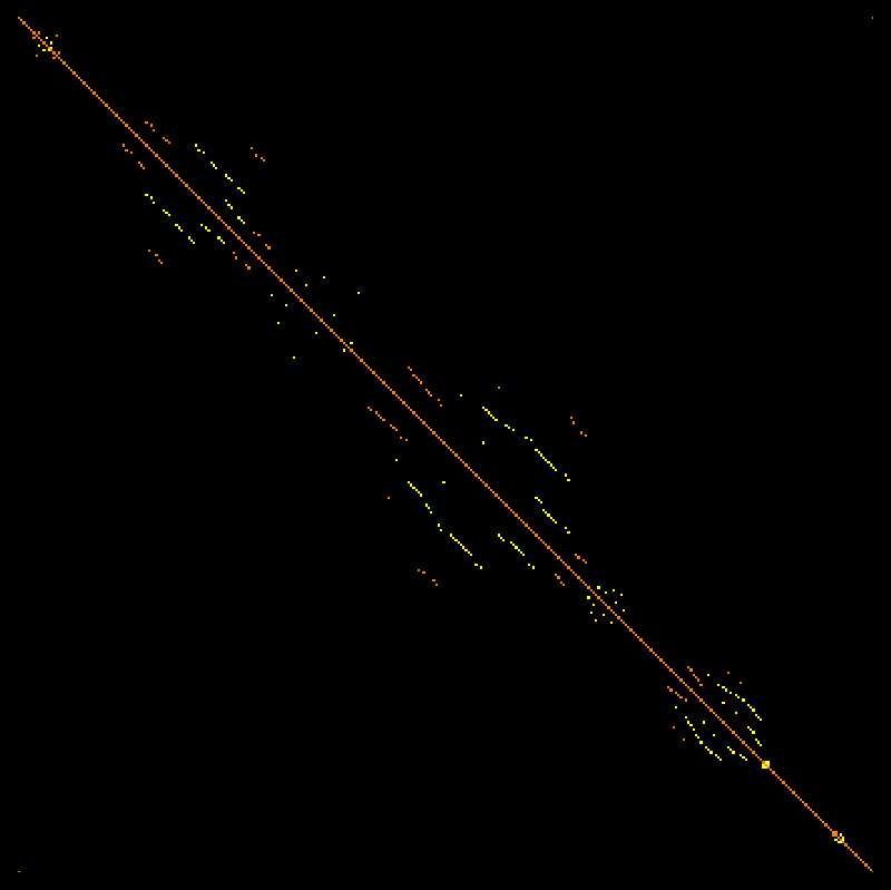
vector) has 5 components. It is (0,0,0,0,0). Here is the Laplacian L of the Wu characteristic of the Moebius graph and then the inverse matrix L-1.
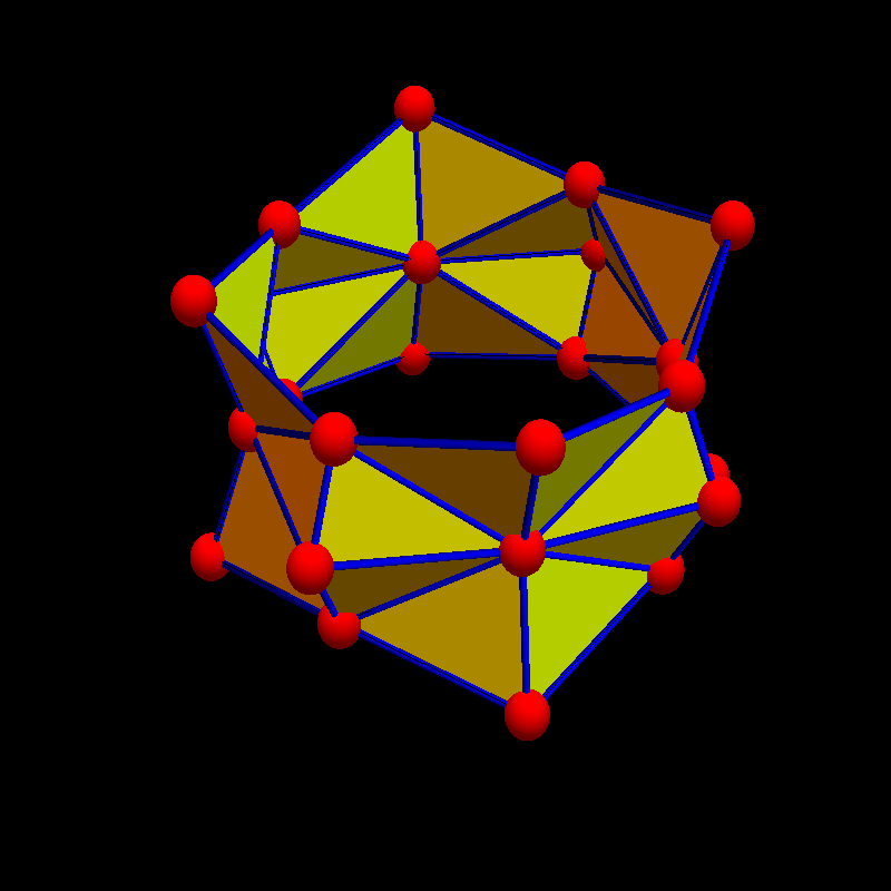
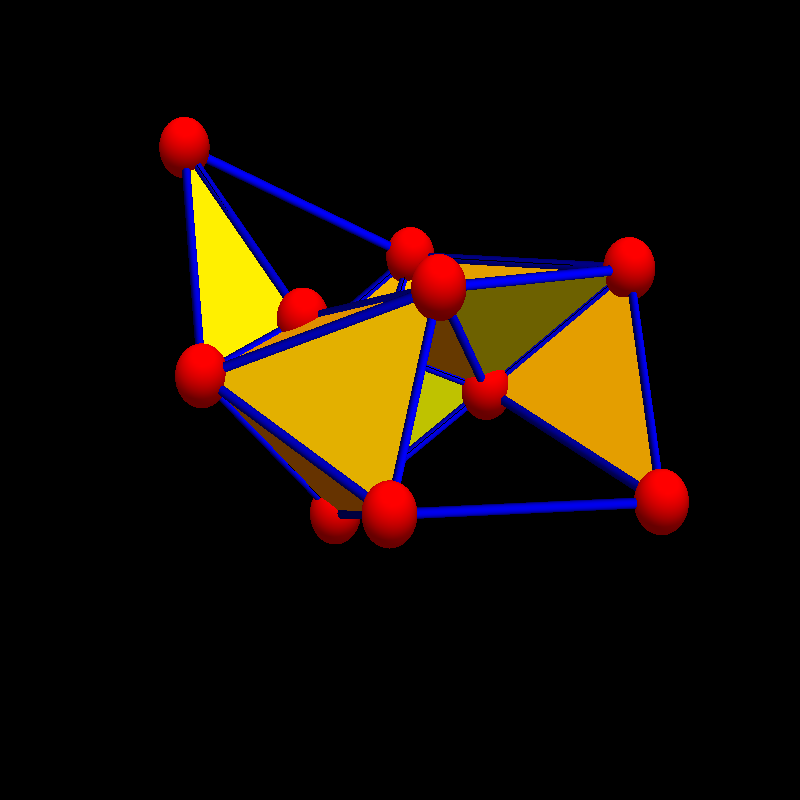
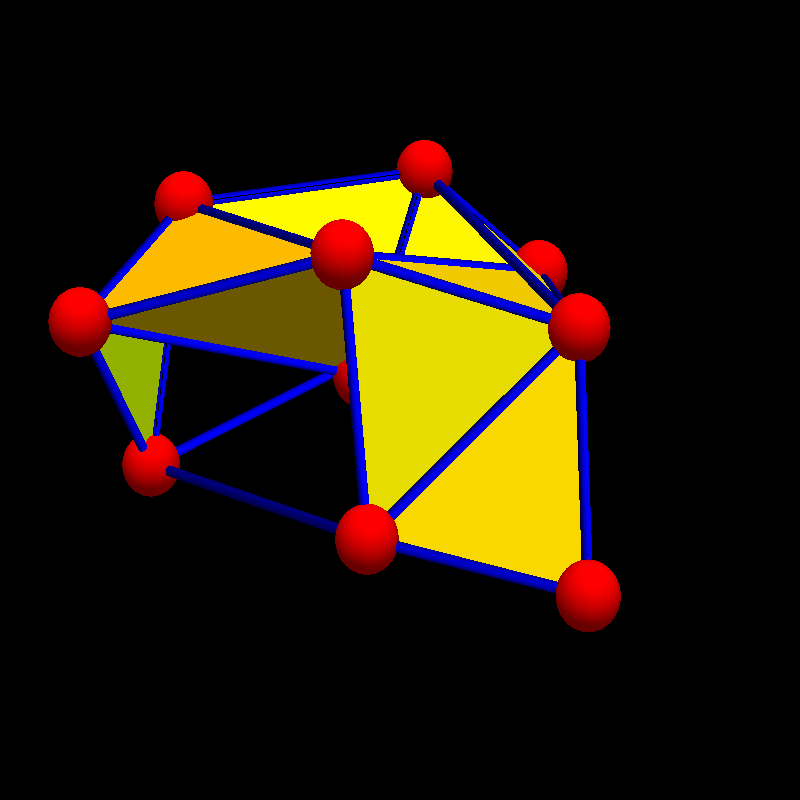
dF(x,y,z) = F(dx,y,z) + (-1)dim(x) F(x,dy,z) + (-1)dim(x)+dim(y) F(x,y,dz) .Here are some computations of the cubic Betti vector, telling about the dimensions of the various cubic interaction cohomology groups. They appear invariant under Barycentric refinement. Of course this still needs to be proven but it should be no problem: just extend the Kuenneth formula to products of graphs. It appears just a technicality to push the chain homotopy construction due to de Rham from the Euler characteristic case (k=1) to the quadratic (k=2), cubic or general k-Wu characteristic case. As in the classical de Rham case, the de Rham construction of cohomology will be a considerable reduction of complexity. De Rham cohomology is considerably less computationally intense than simplicial cohomology, essentially because there are less cubes than simplices needed to cover the geometric structure. However it can only be used if the graph can be patched with charts which have a local product structure (as in manifolds). Complexity reduction is badly needed as the computations of the cohomology groups are getting heavy. In the cubic case, the machine chokes already, when dealing with the relatively small 3-sphere (which is the 16-cell, a Platonic 3-dimensional polytop, a graph with 8 vertices, 24 edges which is classically realized as a convex polytop in 4D and so often dubbed "four dimensional polytop", even so its topological realization is a 3-sphere, a topological 3-manifold). [ Tried first on my Mac Air. But the process even quits due to lack of memory on my office workstation where I always keep the heaviest Thinkmate metal I can afford. The bottle neck is first an innocent looking part which sorts triples of simplices using a built in conditional sort algorithm in Mathematica and then of course linear algebra, where the machine has to deal with 140'816x140'816 matrices. (There are 140'816 ordered triples of intersecting simplices in that graph). To store such a Dirac matrix, one already needs 158 GBytes, which requires a lot of swap space. On my mac air, I have only 8 Gig memory. On my work station (which soon needs to be replaced), I have currently only 32 Gig of RAM. In the next one, I will certainly go to at least 256 Gig of RAM. For now, I might have to deal with less time effective but less memory heavy algorithms or then use theory.] In the following table, the size of the Dirac operator is given to illustrate that linear algebra gets heavy. Bary(G) refers to the Barycentric refinement of G. The Betti vectors for the 3-spheres, 4-spheres, Projective plane and Kleinbottle is what I expect it to be. The projective plane and Klein bottle could be implemented on smaller graphs.
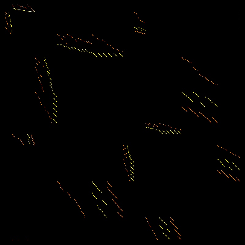
Euler  Betti     Wu3   Cubic Betti          name           Dirac operator
-----------------------------------------------------------------------
  1    (1)       1     (1)                  K_1 (point)            1x1
  0    (1,1)     0     (0,0,1,1)            1-sphere C_4         104x104
  1    (1,0)     1     (0,0,1,0)            K2         15x15
  2    (1,0,1)   2     (0,0,0,0,1,0,1)      2-sphere (octah.)   4058x4058
  2    (1,0,1)   2     (0,0,0,0,1,0,1)      2-sphere (icosah.) 15182x15182
  0    (1,0,0,1) 0     (0,0,0,0,0,0,1,0,0,1)  3-sphere        140816x140816
  2    (1,0,0,0,1) 2   (0,0,0,0,0,0,0,0,1,0,0,0,1)  4-sphere 4583282x4583282
  1    (1,0)     1     (0,0,1,0)            1-ball L(2)           41x41
  1    (1,0,0)   1     (0,0,0,0,1,0,0)      2-ball W(4)         1457x1457
  1    (1,0)    -5     (0,0,0,5)            3-star graph          85x85
  1    (1,0)    -23    (0,0,0,23)           4-star graph         153x153
  1    (1,0)    -59    (0,0,0,59)           5-star graph         251x251
  1    (1,0)    -59    (0,0,0,59)           Bary(5star)          381x381
 -1    (1,2)    -25    (0,0,0,25)           Figure 8 graph       279x279
 -2    (1,3)   -122    (0,0,0,122)          Clover (3 bouquet)   574x574
 -3    (1,4)   -339    (0,0,0,339)          Lucky  (4 bouquet)  1037x1037
 -4    (1,5)   -724    (0,0,0,724)          5 bouquet           1716x1716
 -1    (1,2)    -25    (0,0,0,25)           Bary(Figure8)        487x487
  1    (1,0)     -5    (0,0,0,6,1,0,0)      Rabbit graph         335x335
  1    (1,0)     -5    (0,0,0,6,1,0,0)      Bary(Rabbit)        3651x3651
  0    (1,1)      0    (0,0,0,1,1,0,0)      House graph          342x342
  0    (1,1)      0    (0,0,0,1,1,0,0)      Bary(House)         3672x3672
 -4    (1,5)    -52    (0,0,0,52)           Cube graph           500x500
 -16   (14,30)  -400   (0,0,0,400)          Tesseract           1968x1968
  0    (1,1,0)   0     (0,0,0,0,1,1,0)      Moebius strip       4016x4016
  0    (1,1,0)   0     (0,0,0,0,1,1,0)      Cylinder           12296x12296
  1    (1,0,0)   1     (0,0,0,0,0,0,1)      Projective plane   26953x26953
  0    (1,1,0)   0     (0,0,0,0,0,1,1)      Klein bottle      137100x137100
  1    (1,0,0)   1                          Dunce Hat
Here are pictures of the new Laplacian for the house graph G and its Barycentric refinement G1:

|
|
|

|
| Cubic Dirac G | Cubic Laplacian G | Cubic Dirac G1 | Cubic Laplacian G1 |
dF(x,y) = F(dx,y) + (-1)dim(x) F(x,dy)Here, x,y are the interacting simplices in the graph and dx,dy are the boundary chains and F is a discrete quadratic differential form (or better anti-symmetric quadratic valuation as it is a functional on pairs of oriented subgraphs). All the theorems still work (the heat proof below for Lefschetz for example is so simple and universal that it works for any cohomology given by concrete exterior derivative. This is nice but it seduced to stick with the first best cohomology which came to mind). New is that the cohomology groups are now combinatorial invariants which go over to the continuum. In other words, the Betti numbers are now reasonable. For a triangle for example it is b=(0, 0, 1, 0, 0), for a K4 graph, it is (0,0,0,1,0,0,0) etc. For a circular graphs Cn (the discrete circle) it is (0,1,1). For the octahedron graph (the discrete 2-sphere) (0,0,1,0,1). For the discrete 2-torus, it is (0,0,1,2,1). Lets compute it for list of graphs. For discrete d-manifolds, the Interaction Betti vector is just shifted, adding d zeroes, but for discrete varieties, the numbers are interesting. So, like Wu characteristic, for manifolds, the quantities do not produce any new invariants. This changes however for varieties or more general structures, where the Betti numbers are interesting quantities to study. Also, as there are a couple of cohomologies in the continuum, one has to see whether it belongs to one seen in the continuum.
Euler   Betti       Wu    Interaction-Betti     graph name
-------------------------------------------------------------
  1     (1)         1     (1)                   K1 (point)
  1     (1,0)       -1    (0,1,0)               K2 interval
  0     (1,1)       0     (0,1,1)               1-sphere
  2     (1,0,1)     2     (0,0,1,0,1)           2-sphere
  0     (1,0,0,1)   0     (0,0,0,1,0,0,1)       3-sphere
  2     (1,0,0,0,1) 2     (0,0,0,0,1,0,0,0,1)   4-sphere
  0     (1,2,1)     0     (0,0,1,2,1)           2-torus
  1     (1,0)       -1    (0,1,0)               1-ball
  1     (1,0,0)     1     (0,0,1,0,0)           2-ball
  1     (1,0,0,0)   -1    (0,0,0,1,0,0,0)       3-ball
  1     (1,0)       1     (0,0,1)               3-star graph
  1     (1,0)       1     (0,0,0,0,1)           3-star x 3-star
  1     (1,0)       5     (0,0,5)               4-star graph
  1     (1,0)       11    (0,0,11)              5-star graph
 -1     (1,2)       7     (0,0,7)               Figure 8 graph (w bouquet)
 -2     (1,3)      22     (0,0,22)              Clover (3 bouquet)
 -3     (1,4)      45     (0,0,35)              Lucky  (4 bouquet)
 -4     (1,5)      76     (0,0,76)              5 bouquet
  1     (1,0)       3     (0,0,3,0,0)           Rabbit graph
  0     (1,1)       2     (0,0,2,0,0)           House graph
 -4     (1,5)      20     (0,0,20)              Cube graph
 -16    (14,30)   112     (0,0,112)             Tesseract
  0     (1,1,0)     0     (0,0,0,0,0)           Moebius strip
  0     (1,1,0)     0     (0,0,1,1,0)           Cylinder K2xC4
  0     (1,1,0)     0     (0,0,0,1,1)           Klein bottle
  1     (1,0,0)     1     (0,0,0,0,1)           Projective plane
  1     (1,0,0)     1     (0,0,0,1,2)           Dunce Hat
Here are some computations for random Erdoes-Renyi graphs with 10 vertices. We clearly observe Euler-Poincaré both for Euler characteristic and Wu characteristic: the super sum of the betti numbers are Euler characteristic, the super sum of the interaction betti numbers is the Wu characteristic.
Euler  Betti        Wu     Interaction-Betti
-----------------------------------------------
-3    {1, 4, 0}      5     {0, 0, 6, 1, 0}
-4    {1, 5, 0}     12     {0, 0, 13, 1, 0}
 0    {1, 1, 0, 0}  -6     {0, 0, 1, 7, 0, 0, 0}
-1    {1, 2, 0, 0}  -3     {0, 0, 1, 4, 0, 0, 0}
-2    {1, 3, 0, 0}   2     {0, 0, 3, 1, 0, 0, 0}
-2    {1, 3, 0, 0}   4     {0, 0, 7, 3, 0, 0, 0}
 0    {1, 1, 0, 0}   2     {0, 0, 3, 1, 0, 0, 0}
 0    {1, 1, 0, 0}   2     {0, 0, 3, 2, 1, 0, 0}
-4    {1, 5, 0, 0}  12     {0, 0, 15, 3, 0, 0, 0}
-1    {1, 2, 0, 0}   1     {0, 0, 4, 3, 0, 0, 0}
Here are some larger graphs with 12 vertices:
Euler  Betti           Wu      Interaction-Betti
-----------------------------------------------
-2    {1, 3, 0, 0, 0}   6      {0, 0, 5, 0, 1, 0, 0, 0, 0}
-3    {1, 4, 0, 0}      1      {0, 0, 6, 5, 0, 0, 0}
 1    {1, 2, 2, 0}     -5      {0, 0, 2, 11, 4, 0, 0}
-2    {1, 3, 0, 0}     -4      {0, 0, 3, 7, 0, 0, 0}
-2    {1, 3, 0, 0, 0}   6      {0, 0, 5, 0, 1, 0, 0, 0, 0}
-3    {1, 4, 0, 0}      5      {0, 0, 10, 5, 0, 0, 0}
 0    {1, 1, 0, 0}      2      {0, 0, 1, 0, 1, 0, 0}
 1    {1, 1, 1, 0}     -3      {0, 0, 1, 5, 1, 0, 0}
 2    {1, 0, 1, 0}     -4      {0, 0, 0, 5, 1, 0, 0}
-1    {1, 2, 0, 0, 0}   1      {0, 0, 4, 4, 1, 0, 0, 0, 0}
We still need to implement the cohomology for cubic Wu characteristic.
It certainly will go the same way: define
dF(x,y,z) = F(dx,y,z) + (-1)dim(x) F(x,dy,z) + (-1)dim(x)+dim(y) F(x,y,dz)Now the cubic Wu characteristic will be the super sum of the Interaction betti numbers and the Lefschetz formula will hold.
A benefit of programming the more general Dirac operators is to have rebuilt from scratch the code for computing the standard Dirac operator for simplicial cohomology. The computation of the Betti numbers for an arbitrary simplicial complex is now 12 lines of Mathematica code (the code is displayed at the end of the Dirac paper had been about 18 lines.) To compute it for graphs which have the simplicial complex only impliciely defined, one has to include "Whitney", the procedure to find the Whitney simplicial complex of the graph). The code is now not only more elegant, it also has sped up the computation by a factor 2.
[ By the way, the averaging point of view for curvature is heavily motivated from physics: given a specific "wave" function f, the curvature of space is localized on the Poincaré-Hopf indices. When averaging over all wave functions (a picture of Feynman), we get geometric Euler or more generally Wu curvature. The Feynman picture is omni present in mathematics. Already in the Leibniz definition of determinants where we sum over all closed paths in a complete weighed graph G which is equivalent to summing some action of a path over the automorphism group of G which is the full permutation group. Determinants are a prototype of a path integral. ]
When averaging the Lefschetz numbers iT(x) over all automorphism, this gives a curvature number which has lost its dynamical nature and becomes geometric: it only depends on the graph G. This also works in the Wu characteristic case
sumT in Aut(G) XT,k(G) ,where XT(G) is the Lefschetz number for the T on G for the k-th Wu characteristic. The curvature could be pushed from simplices to vertices as in the proof of the Gauss-Bonnet theorem. In the case when the graph has a trivial automorphism group, the average Lefschetz number is the k'th Wu characteristic of G. In general, it will be the Wu characteristic of a quotient chain. Examples
1) Lets look at it in the case of the graph Cn with n>3, where Aut(G) is a dihedral group. In that case, for any orientation preserving automorphism, the Lefschetz number XT,k(G) is zero and for any orientation reversing automorphism, it is 2. The average is 1.
2) Lets look at the rabbit graph which is also in the handout. All the 4 automorphisms have Lefschetz number 1 (as mentioned in the handout too). We did also compute the Lefschetz numbers with respect to Wu characteristic: the indices are (3, 1, 1, -1), the first one belongs to the identity and agrees with the Wu characteristic of the graph. The average over all Lefschetz numbers is 1.
3) Now lets look at the Wheel graph with 6 spikes. The Automorphism group is the dihedral group D6 and each of the 12 automorphisms has Lefschetz number 1. The Wu-Lefschetz numbers are either 1 or -1. Half of them are minus 1. The average Wu Lefschetz number is 0.
4) For a star graph with 5 spikes, the automorphism group has 5! = 120 elements. The Lefschetz story for Euler characteristic is boring: all 120 automorphisms have the same Lefschetz number 1. The average is 1. For Wu characteristic, there is one automorphism, the identity with Lefschetz number 11, the others are either 1 or -1 and the sum is 0.
5) For the line graph with 4 vertices and 3 edges, the average Lefschetz number is 1, the average Wu Lefschetz number is 0.
5) For the cube graph, the Lefschetz numbers of the 48 automorphisms are (-4, 2, 2, 2, 2, 2, 4, 2, 0, 0, 0, 0, 0, 0, 4, 0, 2, 0, 0, 0, 0, 4, 0, 2, 2, 2, 0, 0, 0, 2, 2, 2, 0, 0, 2, 0, 0, 2, 2, 0, 2, 0, 2, 0, 0, 2, 2, 0) which average to 1. The Wu Lefschetz numbers of the 48 automorphisms are (20,-2, -2, 2, 2, -2, 4, 2, 0, 0, 0, 0, 0, 0, 4, 0, 2, 0, 0, 0, 0, 4, 0, 2, -2, 2, 0, 0, 0, 2, 2, -2, 0, 0, 2, 0, 0, 2, 2, 0, -2, 0, 2, 0, 0, 2, 2, 0), which again averages to 1.
As shown in the fixed point paper, the average Lefschetz number is an integer as it is the Euler characteristic of the quotient chain G/Aut(G) which is not a graph in general. This also holds in the Wu characteristic generalization: The average Lefschetz number of an automorphism is the Wu characteristic of the quotient chain (if we make a Barycentric refinement first, we can assure that the quotient is a graph.
What other numerical quantity could compete? Entropy comes in mind. It is a functional which satisfies many interesting properties like extremal variational properties, explains some central limit theorems in renormalization pictures, where it is a Lyapunov function similarly than energy is in other contexts. The number maximizing entropy -x log(x) is 1/e, where e is the Euler constant 2.718..., somehow showing that e is a most natural number which almost can compete with Pi. And then there are dynamical entropy quantities like topological or metric entropies. They are fair to include as a "dynamical entropy" to the concept "entropy", considering that the Lefschetz number is a "dynamical Euler characteristic". There are a few nice theorems for entropy, especially in ergodic theory or probability theory. It is for example the logarithm of a determinant for some discrete Hamiltonian systems. It is a Lyapunov function under Markov flows. An other candidate for "most important quantity in mathematics" is probably the notion of determinant. Like Euler characteristic, it satisfies a multiplicative property, the Cauchy-Binet formula, even a bit more general. An other candidate could be some values of zeta functions ("quantity" should not include "functions", but numerical quantities, a competition on "functions" would certainly put "Zeta functions" very top). And then there is the notion of "dimension" which also competes rather well as a numerical quantity for geometries. It also satisfies the product formula in many cases or an inequality dim(A x B) >= dim(A) + dim(B), like for Hausdorff dimension and for inductive graph dimension. Other quantities which come to mind are general functionals like probability, energy, action or complexity, the number of Turing computation steps needed for a computation, or the number of proof steps in a predefined axiomatic frame work. Without further structure these notions are however too general to compete. They are so general, that there are not many general theorems for them. So, here is a larger set for candidates for "the most important numerical functional in mathematics":
|
Wu characteristic as a generalization of Euler characteristic certainly has a shot at that list.
|
PROOF: We have a permutation matrix = unitary Koopman transformation U=UT induced by the
graph automorphism on the total interaction Hilbert space of all the simplex interactions in the graph.
And then there is the heat flow V(t) = exp(-t L) which is for every t a matrix of the same size.
Now compose these two transformations to get the heat permutation flow W(t) = U V(t)
and look at its super trace, the trace on the even part minus the trace on the odd part.
For t=0, this trace is nothing else than the sum of the indices of the
fixed interaction k-tuples. Now use the McKean-Singer magic, the super trace of any positive
power of L on the complement of the kernel is always zero.
This is the super symmetry: (See here):
the union of the positive eigenvalues on the even dimensional part of the interaction Laplacian L is the same
than the union of the positive eigenvalues on the odd dimensional part of L.
This symmetry always holds for an operator L = D2, where
D=d+d* with d2=0. The reason is that the Dirac operator D maps between even and
odd dimensional parts and induces an isomorphism on the complement of the harmonic part.
Now, for t reaching to infinity, the heat flow kills the eigen space to the positive eigenvalues and pushes
the operator W(t) towards a projection onto the kernel. The projection onto
harmonic interaction differential forms build the attractor. [March 10: it is maybe still necessary to clarify, why the super trace for t=0 is the sum of the Brouwer indices of the fixed points. First of all, the fixed points are in the diagonal of the Koopman operator, but U also permutes the individual vertices of the fixed simplices. Now if we look at a differential form f (or quadratic differential form f in the Wu case), then permuting the simplex induces a sign change of the form, by definition of differential forms. Together with the super trace definition, every fixed point contributes (-1)dim(x) sign(T|x) or (-1)dim(x)+dim(y) sign(T|x) sign(T|y). ] Since by Hodge theory (which in the discrete just linear algebra because we are in a finite dimensional setup), the kernel of the Laplacian Lm on m-interaction forms parametrized representatives of the m-th cohomology group, the transformation W(infinity) is nothing else than the induced linear transformation on cohomology. Its super trace is by definition the Lefschetz number. In other words,
|
The proof shows that in any situation for which one has Euler Poincaré, there is also a Lefschetz formula for interaction cohomology. The earlier proof in the case of Euler characteristic uses a very simple principle: an action of a permutation on a finite set has two type of invariant sets: either they are cycles or then they are fixed points. The cycles have characteristic zero, the fixed points survive. Note that we have cycles of three points for example, then this is a triangle and counts as a fixed point.
|
Theorem: Lefschetz formula for Wu characteristic: For any graph homomorphism T of a finite simple graph G and any positive k, the Lefschetz number of T with respect to k'th Wu cohomology is the same than the sum of the indices of the fixed interaction k-tuples of T. If T is the identity, then the Lefschetz number is the k'th Wu characteristic and the identity is the Euler-Poincaré formula for Wu characeteristic. For k=1, this is the classical Brouwer-Lefschetz fixed point theorem. |
Note again, we have to stress, that no assumption whatsoever are necessary. The theorem holds for any general finite simple graph = network. Automorphisms are a bit rigid, especially for general networks, the automorphism group is in general rather small. However, the group of homeomorphsims on a graph is much larger. Generalizing Brouwer to a discrete Kakutani theorem was actually the motivation for this paper. In the discrete, graph homeomorphisms are naturally "pointless topological objects" which means when looked upon classically that we have multi-valued maps. This is needed to get any decent version of "homeomorphism" or "rubber geometry" on a graph. Now, in the case of Wu characteristic, there is no proof yet that Wu characteristic is invariant under homeomorphisms. If it should not be the case, I would be even willing to restrict the allowed topologies on graphs or restrict the class of graphs to have it work. [March 10: (one example could be to assume he restriction of having a shellable Whitney complex). It should still be true in general however: it holds for geometric graphs with boundary and if we grow lower dimensional parts, it sill works. And there are certainly non-shellable graphs for which Wu characteristic behaves nicely. Under Barycentric subdivision (which are homeomorphic), the graph grows to a monstrum consisting of patched discrete varieties, something one could visualize a scheme to look like if one would have to make a picture of a scheme. ]
The theorem could be applied in the same way as in classical topology: if the Lefschetz number is not zero, then there are fixed interaction k-tuples. This still needs to be harvested. One would need an application where the interaction between various cliques is of interest and does not change under some transformation. Classical simplicial cohomology gives cliques which are fixed. In the case of Euler characteristic, where one deals with the classical simiplicial cohomology, any transformation on a contractible graph has Lefschetz number 1 and one has the Brouwer fixed point theorem, telling that an automorphism on a contractible graph always has a fixed simplex. Again, as in the case of Euler characteristic, also for Wu characteristic, the Lefschetz formula reduces in the case of the identity just the Euler-Poincaré theorem. Except for very small graphs, examples are hard to compute by hand. Here are two examples. The first one can be done by hand:
Example 1: let G=C4 be the circle graph and T=(4,3,2,1) an orientation reversing transformation. The Euler characteristic and Wu characteristic of G are both zero. The Lefschetz number of T is 2 for Euler characteristic as well as for Wu characteristic: the transformation not only reverses the order of the edges but also the order of edge-vertex interactions. But there are only two fixed points in the Wu chase and both are self interactions of edges by themselves. The index of each of these fixed points is 1. They add up to the Lefschetz number 2.
Example 2: let G be the octahedron graph. It has 6 vertices, 12 edges and 8 triangle. The Hilbert space in which everything works has already dimension 386, which is the sum over all the entries in the f-matrix whose entry Vij encodes how many i-simplices interact with j-simplices:
V(G) = | 6    24   24 |
       |24    84   72 |
       |24    72   56 |
Let the numbering be so that the edge set of G is
E={ (1,2),(1,3),(1,4),(1,5),(2,3),(2,4),(2,6),(3,5),(3,6),(4,5),(4,6),(5,6) }.
Let the transformation be T= {1, 4, 5, 2, 3, 6}. This transformation fixes the
north and south poles 1 and 6 and flips the pairs 2-4 and 3-5.
The traces on the various cohomologies are
{0, 0, -2, 2, 4}
It super sums to 0. Here is a list of fixed pairs of simplices:
fixed interaction       index
-----------------------------
{{1}, {1}}              1
{{1}, {1, 2, 4}}       -1
{{1}, {1, 3, 5}}       -1
{{6}, {6}}              1
{{6}, {2, 4, 6}}       -1
{{6}, {3, 5, 6}}       -1
{{1, 2, 4}, {1}}       -1
{{1, 2, 4}, {1, 2, 4}}  1
{{1, 2, 4}, {1, 3, 5}}  1
{{1, 2, 4}, {2, 4, 6}}  1
{{1, 2, 4}, {2, 4}}    -1
{{1, 3, 5}, {1}}       -1
{{1, 3, 5}, {1, 2, 4}}  1
{{1, 3, 5}, {1, 3, 5}}  1
{{1, 3, 5}, {3, 5, 6}}  1
{{1, 3, 5}, {3, 5}}    -1
{{2, 4, 6}, {6}}       -1
{{2, 4, 6}, {1, 2, 4}}  1
{{2, 4, 6}, {2, 4, 6}}  1
{{2, 4, 6}, {3, 5, 6}}  1
{{2, 4, 6}, {2, 4}}    -1
{{3, 5, 6}, {6}}       -1
{{3, 5, 6}, {1, 3, 5}}  1
{{3, 5, 6}, {2, 4, 6}}  1
{{3, 5, 6}, {3, 5, 6}}  1
{{3, 5, 6}, {3, 5}}    -1
{{2, 4}, {1, 2, 4}}    -1
{{2, 4}, {2, 4, 6}}    -1
{{2, 4}, {2, 4}}        1
{{3, 5}, {1, 3, 5}}    -1
{{3, 5}, {3, 5, 6}}    -1
{{3, 5}, {3, 5}}        1
Also the sum of the indices is zero. Lets compare this with the classical
Lefschetz fixed point formula, where
the transformation T induces a linear map on classical simplicial cohomology,
the traces 1,0,-1 which gives the Lefschetz number 0. Classically, the transformation
has 8 fixed simplices:
fixed simplices        index
----------------------------
{1}                    1
{6}                    1
{1, 4, 2}             -1
{1, 5, 3}             -1
{4, 2, 6}             -1
{5, 3, 6}             -1
{4, 2}                 1
{5, 3}                 1
whose indices add up to zero, the Lefschetz number of the graph automorphism.
|
[ The traditional way to look at the house graph (as Cayley or Coxeter for example would have
seen them) is to look at the "square" as an other face and also include the "outside" as a face
thinking as the graph being on a 2-sphere. When viewed like that, the Euler formula v-e+f=2
would hold. This point of view is problematic in higher dimensions as it produces confusions, what "faces"
are, especially in higher dimensions. As probably best analyzed by Lacatos brilliant analysis
[See Curry's review
PDF]. [Feb 24, 2016: while Lacatos view is different, one can also draw an even more important
conclusion from it (*): definitions are important! Wrong or misleading definitions are as harmful
as wrong or misleading conclusions. Maybe even more as it is hard to find a mistake if different
definitions are used by different mathematicians. If different definitions
appear at the same time detecting errors can be very hard. This in particular appears with the
notion of polyhedron. Other notions which are used in different way are "triangulations".
Fortunately, the notion of a "finite simple graph" does not suffer from this, one reason why
it is a good frame work, to do geometry in. ]
|
(*) An other eloquent exposition about the difficulty was done here by Gruenbaum. His own book on polyhedra wisely just looks at polyhedra which are represented by convex solids in Euclidean space. Here is one of the core points, where Gruenbaum hits the spot:
"How come that results established by such accomplished mathematicians as Euclid, Cauchy, Coxeter, Dress were seemingly disproved after a while? The answer is simple - all the results mentioned are completely valid; what changed is the meaning in which the word "polyhedron" is used."
The Betti vector of G is (1,1,0) and again 1-1+0 = 0, confirming Euler-Poincaré. The eigenvalues of the 0-form Laplacian (the Kirchhoff matrix) is {4.61803, 3.61803, 2.38197, 1.38197, 0}, the eigenvalues of the 1-form Laplacian (the electromagnetic Laplacian) is {4.61803,3.61803,3, 2.38197, 1.38197, 0}. The zero eigenvalue corresponds to a one-dimensional harmonic form winding around the circle. The harmonic eigenvector [3, -3, -2, -1, -3, 1] is naturally the image of the Hurewicz homomorphism from the fundamental group of the graph to the first cohomology group. The 3-form Laplacian is [3] with eigenvalue 3. There is only one triangle. We see the super symmetry: the spectrum on 2-forms and 0-forms together make up the spectrum of 1-forms. That leads to the McKean-Singer formula in graph theory.
Lets now look at the Wu characteristic. The f-matrix is
       | 5   12  3 |
V=     | 12  24  5 |
       | 3   5   1 |   .
The Wu characteristic is (X.V)X, with X=(1,-1,1) which is 2. While the
linear Dirac operator of G is a 12 x 12 matrix, the quadratic Dirac operator D
is a 70 x 70 matrix. The Betti vector of the quadratic cohomology is
{0, 4, 7, 1, 0}
and indeed, b0-b1+b2-b3+b4=0-4+7-1+0=2.
The spectrum of the 0-form Laplacian dealing with the vertex-vertex interactions is {3, 3, 2, 2, 2}
(where we see no cohomological obstructions)
the spectrum of the 1-form Laplacian dealing with vertex-edge interactions is
{4,3.61803,3.61803,3.61803,3.61803,3,3,3,2,2,2,2,2,2,2,1.38197,1.38197,1.38197,1.38197,1,0,0,0,0}
(with a 4 dimensional kernel) the spectrum of the 2-form Laplacian dealing with edge-edge and
triangle-point interactions is
{4,4,3.61803,3.61803,3.61803,3.61803,3.41421,3,3,3,3,2,2,2,2,2,2,1.38197,1.38197,1.38197,1.38197,
1,0.585786,0,0,0,0,0,0,0} (with a 7 dimensional kernel).
The spectrum of the 3-form Laplacian dealing with edge-triangle interactions
is {4,3.41421,3,3,3,3,2,2,0.585786,0} and the spectrum
of the 4-form Laplacian dealing with triangle-triangle interactions is {3}. Nicely confirmed is
supersymmetry which means that every nonzero eigenvalue for an even form (Bosonic) Laplacian
appears as an eigenvalue of an odd form (Fermionic) Laplacian and vice versa.
|
We still don't know what the harmonic forms represent. As always in cohomology they are obstructions
to the solutions of some equations, in this case coming by the interactions of the various pieces
of geometry. Some cocycles F (satisfying dF(A,B)=0) are not coboundaries (satisfying dG(A,B) = G(dA,B) ).
They are represented by kernel elements of the corresponding Laplacians. What are these harmonic forms?
In the case of edge-vertex interactions, (1-forms)
they come from interactions at the vertices where the triangle is attached.
In the case of the edge-edge or triangle vertex interactions (1+1 forms or 2+0 forms) there is
a seven dimensional space of obstructions. As mentioned already, these obstructions are not
geometric, because they change with Barycentric refinement. The Betti vector for discrete quadratic
differential forms is
{0, 7, 13, 4, 0}
The super sum is still 2 but the cohomology has changed. By the way, quadratic Dirac operator for
the Barycentric refinement is already a 378x378 matrix even-so the graph has only 12 vertices and 18 edges
and 6 triangles.
|
For the cubic Wu characteristic, we need to look at the f-tensor
                     5    12   3
                     12   30   8
                     3    8    3

V =                  12   30   8
                     30   72   19
                     8    19   5

                     3    8    3
                     8    19   5
                     3    5    1
The cubic Wu characteristic is ((V.X).X).X which is here 0.
The Dirac operator of the cubic differential forms is a 342x342 matrix. The cubic Betti vector is
{0, 4, 20, 27, 12, 1, 0}
whose super sum is 0+20+12-4-27 -1=0. This is Euler-Poincaré for the cubic Wu characteristic.
While the cubic Wu characteristic
w3(G) = sumx,y,z w(x) w(y) w(z)summing over all triples of intersecting simplices in the graph G is also invariant under Barycentric refinement (even satisfies the product formula), also the cubic interaction obstruction numbers bk (= Betti numbers for cubic cohomology) change under Barycentric refinement. The cubic Dirac operator D=d+d* of the Barycentric refinement G1 of the house graph G is already a 3672x3672 matrix. Here is the cubic Betti vector of that Barycentric refinement:
{0, 7, 37, 66, 74, 56, 18}
Interestingly, as there is now more than one triangle, there are also interaction obstructions
for the 6 triangles.
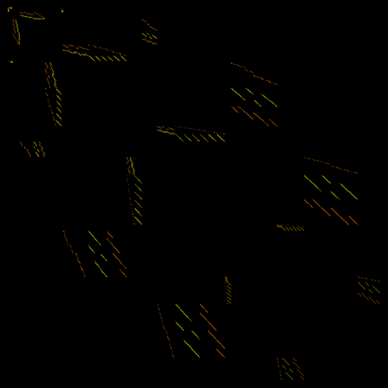
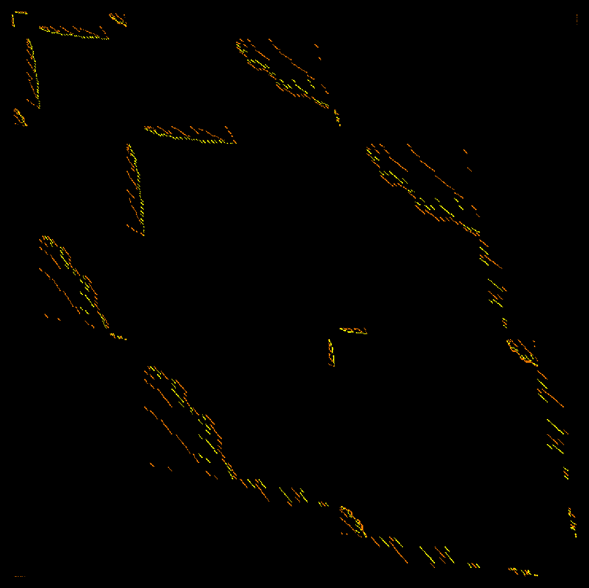
Here are pictures of the Dirac operator, quadratic Dirac operator and cubic Dirac operator

|

|

|
|
|
|

|
|
|
|
|
|
- There is a Euler Poincaré formula. The Wu characteristic is the alternating sum of the Betti number of the cohomology. The proof is identical and basic linear algebra. Essentially the Rank-Nullety theorem (which by accident will is taught this week in our Math21b course.
- The form Laplacian (d+d*)2 satisfies the McKean-Singer formula. The proof is identical to the proof for the standard cohomology. There is super symmetry. The story is completely parallel to The McKean-Singer formula for standard cohomology.
- Also identical is the Hodge story. The cohomology groups are isomorphic as vector spaces to the space of harmonic forms of the corresponding form Laplacians. We don't have a feel yet what the harmonic forms really mean. Since they are not topological and change under deformation, this might be more difficult to answer. But they certainly play a role when looking at wave, heat or other PDE dynamics related to the new Laplacian as these are stationary states. Whether this wave dynamics is physically interesting is not clear yet. I personally do not doubt this for a moment. Any Laplacian defined through exterior derivatives has turned out to be interesting. This one might be a bit exotic. But fundamental basic physics is exotic.
- Also the isospectral deformation of the new Dirac operator defines still an integrable system. It deforms the intersection cohomology by isospectrally deforming the exterior derivative. We did not check the details but believe the story to be similar and that the dynamics produces an inflationary start and expansion of geometry.
- Unlike the standard cohomolgy, the cohomology groups change with homotopy deformations. A bit disappointing: the cohomology also changes when doing Barycentric refinement. We can not expect the groups to be relevant in the continuum limit therefore. Anyway, there does not seem to be anything like that in the continuum. Intersection homology of Goresky and MacPherson for example looks very different. But this intersection cohomology is one of infinitely many cohomologies one can define for graphs (this is the quadratic one, one can also look at cubic versions and higher order versions in exactly the same way by looking at the exterior derivative dF(A,G,G,...,G) = F(dA,G,G,...G) For every of the Wu characteristic wk(G), there are cohomology groups Hkn. I might implement the cubic one to see whether there is something going on.
 |
 |
| Proposition (Reti): Among all trees, the Wu characteristic is maximized by star graphs and minimized by line graphs. |
|
Lemma (Reti) For a triangle free graph with n vertices and m edges, the Wu characteristic is n-5m+M(G) where M(G) is the first Zagreb index, |
A corollary also stated by Tamas Reti is
| For triangle free graphs, the degree sequences alone completely determine the Wu characteristic. |
|
Alternatively, one can see the corollary also from the fact that
Barycentric refinement separates the singularities
and the fact that the degree of a singularity determines
the type of singularity if the graph has no triangles. The Zagreb indices seem to be really nice and relevant in Mathematical chemistry, where it seems have been quite useful. |
| The Wu embedding number of a single point v in a graph is the Euler-Poincaré index of a function f which has the vertex v as a maximum! |
Now, as explored a bit in this article on Graphs in Eulerian unit spheres, the dual graph of a simplex x in a geometric graph is the intersection of spheres and so a sphere. This is an almost trivial statement but important here too. As we can see that if A is a k-simplex in a geometric d-graph then w(A,G) = (-1)d-k. Super cool, since we have now the general formula
| w(A,G) = (-1)d X(A) if G is a d-graph. |
In the special case if A=G, then this reduces to w(G) = (-1)^d X(G). But stop, is this not a contradiction to the formula w(G) = X(G) which we have proven for d-graphs? Actually not. It reproves that X(G)=0 for odd dimensional graphs!
| Now, I must admit that I would have been much more excited if the embedding number w(A,G) would have produced some interesting numbers. Initially, I was looking for closed curves A in 3-spheres G, objects which are also called knots. Wouldn't it have been cool too if the number w(A,G) would be a number which is homotopy invariant but depend on how the knot is embedded? It would give a knot invariant. Actually, I was looking at this question experimentally before getting into the theory and had the disappointment already seen there. The answer had always been zero. But it had been clear already before looking that both scenarios are interesting, the situation that it does not depend on the embedding, and the situation that it does depend on the embedding. |
 In the fall of 2015, we had also asked students to generate knots.
This one is by Nari Yoon.
In the fall of 2015, we had also asked students to generate knots.
This one is by Nari Yoon.
|
(* indices of barycentric characteristic as defined  *)
BIndices0[f_,s_]:=Module[{a,b,V,A,B,d,VL,v,X,H},
  VL=VertexList[s]; d=CliqueNumber[s]; Table[ X=Bvector[k,d];
  Table[a={};b={};v=VL[[l]]; V=VertexList[NeighborhoodGraph[s,v]];
  Do[If[f[[V[[i]]]] Length[B],0,B[[j]]*X[[j]]]
    - If[j>Length[A],0,A[[j]]*X[[j]]],{j,d}],{l,Length[VL]}],{k,d}]];

(* Bindices done differently: chip fire  *)
BIndices[f_,s_]:=Module[{d=CliqueNumber[s],c=Whitney[s],v,m},
Table[X=Bvector[k,d];a=Table[0,{Length[VertexList[s]]}];
Do[u=c[[l]]; ff=Table[f[[u[[j]]]],{j,Length[u]}];
 m=Max[ff];t=Position[f,m][[1,1]];a[[t]]+=X[[Length[u]]],
{l,Length[c]}];a,{k,1,d}]];
Here is an example. Lets take the 2-sphere given by the Octahedron graph.
As it is 2-dimensional, of course, the clique number is 3. The three
Barycentric vectors are (1,-1,1), (0,2,-3), (0,0,1) called Euler characteristic,
Boundary valuation and volume. Take the function f=(1,2,3,4,5,6)
s=sphere2; d=CliqueNumber[s];
f=Range[Length[VertexList[s]]];
BIndices[f,s]
gives
{{1, 0, 0, 0, 0, 1},
 {0, 2, 1, 1, 0, -4},
 {0, 0, 1, 1, 2, 4}}
You see that the function f is a nice Morse function with 2 critical points
of index 1. This is of course the maximum and minimum of f. There are no saddles.
The boundary indices add up to 0, which is a trivial case of the Dehn-Sommerville
relations. It reflects that the graph is a 2-graph without boundary.
Finally, the last valuation, the volume gives indices 1,1,2,4 which add up to 8,
the number of triangles of the octahedron. The Barycentric characteristic functions
of the Octahedron are (2,0,8), and we have computed the Poincaré-Hopf indices
which add up to each of these values.
Since G is regular, the curvatures are constant. They are constant 1/3 for the
Euler characteristic, constant 0 for the Boundary valuation and 4/3 for volume. In
general, volume curvature at a vertex v is the face degree at v divided by 3.
If you want to try this out yourself (all the code is available on the LaTeX source)
try to find a function f, on the 2-sphere for which there are two maxima, one minimum
and one saddle point. Try RFunction, which produces a random function on the graph.
BIndices[RFunction[s],s]Here are some exercises. The possibilities are endless.
- Show that on the octahedron graph the Poincaré-Hopf indices of a vertex are always either 0 or 1 or -1.
- Construct an example of a 2-sphere and a function f for which the index at at some vertex is -2. (this is the discrete case of a Monkey-Saddle! We need a larger graph than an octahedron in view of the previous problem.)
- Verify that the Poincaré-Hopf indices of volume are always non-negative.
- Verify that in the case of the Octahedron, the Poincaré-Hopf indices of the volume valuation are supported always on at least 2 vertices.
- Construct a graph and a function for which the Poincaré-Hopf index of the volume is located on one point only.
- What is the Boundary valuation in the case of a wheel graph of volume n?
- The term combinatorial invariant should be used consistently instead of topological invariant. The reason is that having a quantity which is invariant under Barycentric refinement does not necessarily mean to have a quantity which is invariant under homeomorphisms It is still possible that the Wu characteristic becomes a topological invariant but this is not yet proven. While obvious for Euler characteristic, it is not yet proven that Wu characteristic is invariant under homeomorphisms.
- As a corollary of the boundary formula we can only conclude that for
manifolds without boundary, the Wu and Euler characteristic agree.
For even dimensional graphs with boundary, we can glue two copies along the
boundary and see that the Euler characteristic and the Wu characteristic agree.
An example is the 2-disc where the Wu and Euler characteristic is 1, half of
the value of the sphere.
For an odd dimensional graph with boundary, gluing gives an odd dimensional graph
without boundary for which the Euler and Wu characteristic are both zero.
The Wu characteristic is then minus half of the Euler characteristic of the boundary.
- In figure 14, the Wu characteristic of the torus is of course 0 not 1.
By the way, this torus G has been obtained with
GraphProduct[CycleGraph[4],CycleGraph[4]]
a 2-graph with 64 vertices and 192 edges and 128 triangles. It is shown to the right. Its f-vector is v={64,192,128), its f-matrix is [[64, 384, 384], [384, 2368, 2176], [384, 2176, 1920]]. - There were no examples yet of Poincaré-Hopf and index expectation
for general valuations. For Poincaré-Hopf only the old proof was given.
When looking at the general result, the proof is even easier (the above code illustrates
it): given a function f, take the values of the valuation on the simplices x and
"fire" them to the vertex of the simplex where f is maximal. This immediately
shows why the Poincaré-Hopf index of a general valuation at a vertex v of the graph
is the formula
X(B-fv) - X(S- f(v)because this counts the valuations up from all simplices attached to v on which f(v) is maximal. Here is an amusing example: the index to the volume valuation X=vd counting the number of simplices of maximal dimension has the index if(v) counting the number of facets, for which f(v) is the maximum on the simplex. - in the explanation why the addition (V,E)+(W,F) = (F+W,E+F) of finite simple graphs is only a chain there had been a typo in( {1,2},{(12)} ) + ( {2,3},{(23)} ) = ({1,3},{(12),(23)}) which is not a graph as for a graph (V,E), the union of the vertices in E has to be a subset of V. Here is more elaboration why the lack of a linear structure on the category of graphs makes the evaluation of valuations is an important issue: assume we had a Boolean linear algebra structure on graphs, then we could use the valuations on a basis to compute the valuation on any graph. The computations would be polynomial.
- dimensions missing when mentioning Betti numbers b0,b1.
