Oliver Knill
Probability theory is a fundamental pillar of modern mathematics with
relations to other mathematical areas like algebra, topology, analysis,
geometry or dynamical systems. As with any fundamental mathematical construction, the theory
starts by adding more structure to a set  . In a similar way as introducing
algebraic operations, a topology, or a time evolution on a set, probability theory
adds a measure theoretical structure to which generalizes "counting" on
finite sets: in order to measure the probability of a subset
. In a similar way as introducing
algebraic operations, a topology, or a time evolution on a set, probability theory
adds a measure theoretical structure to which generalizes "counting" on
finite sets: in order to measure the probability of a subset
 , one
singles out a class of subsets
, one
singles out a class of subsets  , on which one can hope to do so.
This leads to the notion of a
, on which one can hope to do so.
This leads to the notion of a  -algebra . It is a set of subsets of
in which on can perform finitely or countably many operations like
taking unions, complements or intersections.
The elements in are called events. If a point
-algebra . It is a set of subsets of
in which on can perform finitely or countably many operations like
taking unions, complements or intersections.
The elements in are called events. If a point  in the "laboratory"
denotes an "experiment", an "event"
in the "laboratory"
denotes an "experiment", an "event"  is a subset of , for which
one can assign a probability
is a subset of , for which
one can assign a probability
![$\Prob[A] \in [0,1]$](images/img7.png) . For example, if
. For example, if
![$\Prob[A]=1/3$](images/img8.png) , the event happens with probability
, the event happens with probability  .
If
.
If ![$\Prob[A]=1$](images/img10.png) , the event takes place almost certainly. The probability
measure
, the event takes place almost certainly. The probability
measure  has to satisfy obvious properties like that the union
  of two
disjoint events
of two
disjoint events  satisfies
![$\Prob[A \cup B]
= \Prob[A] + \Prob[B]$](images/img14.png) or that the complement
or that the complement  of an event
  has the probability
![$\Prob[A^c]=1-\Prob[A]$](images/img17.png) .
With a probability space
.
With a probability space
 alone, there is already some interesting mathematics:
one has for example the combinatorial problem to find the probabilities of events
like the event to get a "royal flush" in poker.
If is a subset of an Euclidean space like the plane,
alone, there is already some interesting mathematics:
one has for example the combinatorial problem to find the probabilities of events
like the event to get a "royal flush" in poker.
If is a subset of an Euclidean space like the plane,
![$\Prob[A] = \int_A f(x,y) \; dx dy$](images/img19.png) for a suitable nonnegative function
for a suitable nonnegative function  , we are led to integration problems
in calculus. Actually, in many applications, the probability space is part of
Euclidean space and the -algebra is the smallest
which contains all open sets. It is called the Borel -algebra.
An important example is the Borel -algebra on the real line.
, we are led to integration problems
in calculus. Actually, in many applications, the probability space is part of
Euclidean space and the -algebra is the smallest
which contains all open sets. It is called the Borel -algebra.
An important example is the Borel -algebra on the real line.
Given a probability space
, one can define random variables  .
A random variable is a function from to the real line
.
A random variable is a function from to the real line  which is measurable
in the sense that the inverse of a measurable Borel set
which is measurable
in the sense that the inverse of a measurable Borel set  in is in .
The interpretation is that if is an experiment, then
in is in .
The interpretation is that if is an experiment, then  measures an
observable quantity of the experiment.
The technical condition of measurability resembles the notion of a continuity for a
function from a topological space
measures an
observable quantity of the experiment.
The technical condition of measurability resembles the notion of a continuity for a
function from a topological space
 to the topological
space
to the topological
space  . A function is continuous if
 for all open sets
  .
In probability theory, where functions are often denoted with capital letters, like
.
In probability theory, where functions are often denoted with capital letters, like  ,
a random variable is measurable if
,
a random variable is measurable if
 for all Borel sets
  .
Any continuous function is measurable for the Borel -algebra. As in calculus, where
one does not have to worry about continuity most of the time, also in probability theory, one
often does not have to sweat about measurability issues. Indeed, one could suspect that notions like
-algebras or measurability were introduced by mathematicians to scare
normal folks away from their realms. This is not the case. Serious issues are avoided with those constructions.
Mathematics is eternal: a once established result will be true also
in thousands of years. A theory in which one could prove a theorem as well as its negation would be worthless:
it would formally allow to prove any other result, whether true or false. So, these notions
are not only introduced to keep the theory "clean", they are essential for the "survival" of the theory.
We give some examples of "paradoxes" to illustrate the need for building a careful theory.
Back to the fundamental notion of random variables: because they are just
functions, one can add and multiply them by defining
.
Any continuous function is measurable for the Borel -algebra. As in calculus, where
one does not have to worry about continuity most of the time, also in probability theory, one
often does not have to sweat about measurability issues. Indeed, one could suspect that notions like
-algebras or measurability were introduced by mathematicians to scare
normal folks away from their realms. This is not the case. Serious issues are avoided with those constructions.
Mathematics is eternal: a once established result will be true also
in thousands of years. A theory in which one could prove a theorem as well as its negation would be worthless:
it would formally allow to prove any other result, whether true or false. So, these notions
are not only introduced to keep the theory "clean", they are essential for the "survival" of the theory.
We give some examples of "paradoxes" to illustrate the need for building a careful theory.
Back to the fundamental notion of random variables: because they are just
functions, one can add and multiply them by defining
 or
or
 . Random variables form so an algebra
  .
The expectation of a random variable is denoted by
.
The expectation of a random variable is denoted by ![$\E[X]$](images/img35.png) if it exists. It is a real number
which indicates the "mean" or "average" of the observation . It is the value, one would expect
to measure in the experiment. If
if it exists. It is a real number
which indicates the "mean" or "average" of the observation . It is the value, one would expect
to measure in the experiment. If  is the random variable which has the value
 if is in the
event and
if is in the
event and  if is not in the event , then the expectation of is just the
probability of . The constant random variable
if is not in the event , then the expectation of is just the
probability of . The constant random variable  has the expectation
 ![$\E[X]=a$](images/img40.png) .
These two basic examples as well as the linearity requirement
.
These two basic examples as well as the linearity requirement
![$\E[a X + b Y]= a \E[X] + b \E[Y]$](images/img41.png) determine the
expectation for all random variables in the algebra :
first one defines expectation for finite sums
determine the
expectation for all random variables in the algebra :
first one defines expectation for finite sums
 called
elementary random variables,
which approximate general measurable functions. Extending the expectation to a subset
called
elementary random variables,
which approximate general measurable functions. Extending the expectation to a subset  of the entire algebra is part of integration theory. While in calculus,
one can live with the Riemann integral on the real line,
which defines the integral by Riemann sums
of the entire algebra is part of integration theory. While in calculus,
one can live with the Riemann integral on the real line,
which defines the integral by Riemann sums
![$\int_a^b f(x) \; dx \sim \frac{1}{n} \sum_{i/n \in [a,b]} f(i/n)$](images/img44.png) , the integral
defined in measure theory is the Lebesgue integral. The later is
more fundamental and probability theory
is a major motivator for using it. It allows to make statements like that the
probability of the set of real numbers with periodic decimal expansion
has probability . In general, the probability of
is the expectation of the random variable
, the integral
defined in measure theory is the Lebesgue integral. The later is
more fundamental and probability theory
is a major motivator for using it. It allows to make statements like that the
probability of the set of real numbers with periodic decimal expansion
has probability . In general, the probability of
is the expectation of the random variable
 .
In calculus, the integral
.
In calculus, the integral
 would not be defined because a Riemann integral can
give or depending on how the Riemann approximation is done.
Probability theory allows to introduce the Lebesgue integral
by defining
would not be defined because a Riemann integral can
give or depending on how the Riemann approximation is done.
Probability theory allows to introduce the Lebesgue integral
by defining
 as the limit of
 for
for  , where
 are random uniformly distributed points in the interval
 ![$[a,b]$](images/img51.png) . This Monte Carlo
definition of the Lebesgue integral is based on the law of large numbers and is
as intuitive to state as the Riemann integral
which is the limit of
. This Monte Carlo
definition of the Lebesgue integral is based on the law of large numbers and is
as intuitive to state as the Riemann integral
which is the limit of
![$\frac{1}{n} \sum_{x_j=j/n \in [a,b]} f(x_j)$](images/img52.png) for .
for .
With the fundamental notion of expectation one can define the variance,
![$\Var[X] = \E[X^2]-\E[X]^2$](images/img53.png) and the standard deviation
and the standard deviation
![$\sigma[X] = \sqrt{\Var[X]}$](images/img54.png) of a random variable for which
of a random variable for which
 . One can also look at the
covariance
. One can also look at the
covariance
![$\Cov[X Y] = \E[X Y] - \E[X] \E[Y]$](images/img56.png) of two random variables
of two random variables  for which
 . The correlation
![$\Corr[X,Y] = \Cov[X Y]/(\sigma[X] \sigma[Y])$](images/img59.png) of
two random variables with positive variance is a number which tells how much the random variable
is related to the random variable
of
two random variables with positive variance is a number which tells how much the random variable
is related to the random variable  . If
. If ![$\E[X Y]$](images/img61.png) is interpreted as an inner product, then the
standard deviation is the length of
is interpreted as an inner product, then the
standard deviation is the length of ![$X-\E[X]$](images/img62.png) and the
correlation has the geometric interpretation as
and the
correlation has the geometric interpretation as  , where
 is the angle between the centered random variables
and
is the angle between the centered random variables
and ![$Y-\E[Y]$](images/img65.png) .
For example, if
.
For example, if ![$\Cov[X,Y]=1$](images/img66.png) , then
, then  for some
  , if
, if ![$\Cov[X,Y]=-1$](images/img69.png) , they
are anti-parallel. If the correlation is zero, the geometric interpretation is
that the two random variables are perpendicular. Decorrelated random variables still can have relations
to each other but if for any measurable real functions and
, they
are anti-parallel. If the correlation is zero, the geometric interpretation is
that the two random variables are perpendicular. Decorrelated random variables still can have relations
to each other but if for any measurable real functions and  , the random variables
 and
and  are uncorrelated, then the random variables are independent.
A random variable can be described well by its distribution function
 . This is a real-valued function defined as
![$F_X(s) = \Prob[ X \leq s ]$](images/img74.png) on , where
on , where
 is the event of all experiments satisfying
 . The distribution
function does not encode the internal structure of the random variable ; it does not reveal the
structure of the probability space for example.
But the function allows the construction of a probability space with
exactly this distribution function. There are two important types of distributions, continuous
distributions with a probability density function
. The distribution
function does not encode the internal structure of the random variable ; it does not reveal the
structure of the probability space for example.
But the function allows the construction of a probability space with
exactly this distribution function. There are two important types of distributions, continuous
distributions with a probability density function  and discrete distributions
for which
and discrete distributions
for which  is piecewise constant. An example of a continuous distribution is
the standard normal distribution, where
is piecewise constant. An example of a continuous distribution is
the standard normal distribution, where
 . One can characterize it
as the distribution with maximal entropy
. One can characterize it
as the distribution with maximal entropy
 among all distributions which have zero mean and variance . An example of a discrete
distribution is the Poisson distribution
among all distributions which have zero mean and variance . An example of a discrete
distribution is the Poisson distribution
![$\Prob[X=k] = e^{-\lambda} \frac{\lambda^k}{k!}$](images/img81.png) on
on
 .
One can describe random variables by their moment generating functions
.
One can describe random variables by their moment generating functions
![$M_X(t) = \E[e^{X t}]$](images/img83.png) or
by their characteristic function
or
by their characteristic function
![$\phi_X(t) = \E[e^{i X t}]$](images/img84.png) . The later is the
Fourier transform of the law
. The later is the
Fourier transform of the law  which is a measure on the real line .
The law  of the random variable is a probability measure on the real line satisfying
![$\mu_X( (a,b] ) = F_X(b)-F_X(a)$](images/img87.png) . By the
Lebesgue decomposition theorem, one can decompose any measure
. By the
Lebesgue decomposition theorem, one can decompose any measure  into a discrete part
  ,
an absolutely continuous part
,
an absolutely continuous part  and a singular continuous part
  .
Random variables for which is a discrete measure are called discrete random variables,
random variables with a continuous law are called continuous random variables. Traditionally,
these two type of random variables are the most important ones. But singular continuous random variables
appear too: in spectral theory, dynamical systems or fractal geometry.
Of course, the law of a random variable does not need to be pure. It can mix the three types.
A random variable can be mixed discrete and continuous for example.
.
Random variables for which is a discrete measure are called discrete random variables,
random variables with a continuous law are called continuous random variables. Traditionally,
these two type of random variables are the most important ones. But singular continuous random variables
appear too: in spectral theory, dynamical systems or fractal geometry.
Of course, the law of a random variable does not need to be pure. It can mix the three types.
A random variable can be mixed discrete and continuous for example.
Inequalities play an important role in probability theory.
The Chebychev inequality
![$\Prob[\vert X-\E[X]\vert \geq c] \leq \frac{\Var[X]}{c^2}$](images/img92.png) is used very often. It is a special case of the Chebychev-Markov inequality
is used very often. It is a special case of the Chebychev-Markov inequality
![$h(c) \cdot \Prob[X \geq c] \leq \E[h(X)]$](images/img93.png) for monotone nonnegative functions
for monotone nonnegative functions  .
Other inequalities are the Jensen inequality
.
Other inequalities are the Jensen inequality
![$\E[h(X)] \geq h(\E[X])$](images/img95.png) for convex functions ,
the Minkowski inequality
for convex functions ,
the Minkowski inequality
 or
the Hölder inequality
or
the Hölder inequality
 for random variables, , for which
![$\vert\vert X\vert\vert _p=\E[\vert X\vert^p], \vert\vert Y\vert\vert _q=\E[\vert Y\vert^q]$](images/img98.png) are finite. Any inequality which appears in analysis can be useful
in the toolbox of probability theory.
are finite. Any inequality which appears in analysis can be useful
in the toolbox of probability theory.
Independence is an central notion in probability theory. Two events are called
independent, if
![$\Prob[A \cap B] = \Prob[A] \cdot \Prob[B]$](images/img99.png) . An arbitrary set of events
. An arbitrary set of events  is
called independent, if for any finite subset of them, the probability of their intersection
is the product of their probabilities. Two -algebras
is
called independent, if for any finite subset of them, the probability of their intersection
is the product of their probabilities. Two -algebras  are called
independent, if for any pair
are called
independent, if for any pair
 , the events are
independent. Two random variables are independent, if they generate independent
-algebras. It is enough to check that the events
, the events are
independent. Two random variables are independent, if they generate independent
-algebras. It is enough to check that the events
 and
and
 are independent for all intervals
  and
and  . One should think of
independent random variables as two aspects of the laboratory which do not influence each other.
Each event
. One should think of
independent random variables as two aspects of the laboratory which do not influence each other.
Each event
 is independent of the event
 .
While the distribution function
.
While the distribution function  of the sum of two independent random variables is a convolution
 ,
the moment generating functions and characteristic functions satisfy the formulas
,
the moment generating functions and characteristic functions satisfy the formulas
 and
and
 . These identities
make
. These identities
make  valuable tools to compute the distribution of
an arbitrary finite sum of independent random variables.
valuable tools to compute the distribution of
an arbitrary finite sum of independent random variables.
Independence can also be explained using conditional probability
with respect to an event of positive probability: the
conditional probability
![$\Prob[A \vert B] = \Prob[A \cap B]/\Prob[B]$](images/img114.png) of is the probability that happens when we know that takes place.
If is independent of , then
of is the probability that happens when we know that takes place.
If is independent of , then
![$\Prob[A\vert B] = \Prob[A]$](images/img115.png) but in general, the
conditional probability is larger.
The notion of conditional probability leads to the important notion of conditional expectation
but in general, the
conditional probability is larger.
The notion of conditional probability leads to the important notion of conditional expectation
![$\E[X \vert \Bcal]$](images/img116.png) of a random variable with respect to some sub--algebra
of a random variable with respect to some sub--algebra  of the
algebra ; it is a new
random variable which is -measurable. For
of the
algebra ; it is a new
random variable which is -measurable. For  , it is the random variable itself,
for the trivial algebra
, it is the random variable itself,
for the trivial algebra
 , we obtain the usual expectation
![$\E[X] = \E[X \vert \{\emptyset,\Omega \;\}]$](images/img120.png) . If
is generated by a finite partition
. If
is generated by a finite partition
 of of pairwise disjoint sets covering
, then is piecewise constant on the sets
of of pairwise disjoint sets covering
, then is piecewise constant on the sets  and the value on is
the average value of on . If is the -algebra of an independent random
variable , then
and the value on is
the average value of on . If is the -algebra of an independent random
variable , then
![$\E[X \vert Y ] = \E[X \vert \Bcal] = \E[X]$](images/img123.png) . In general, the
conditional expectation with respect to is a new random variable obtained by averaging
on the elements of . One has
. In general, the
conditional expectation with respect to is a new random variable obtained by averaging
on the elements of . One has
![$\E[X \vert Y ]=h(Y)$](images/img124.png) for some function , extreme cases being
for some function , extreme cases being
![$\E[X \vert 1] = \E[X], \E[X \vert X] = X$](images/img125.png) .
An illustrative example is the situation where
.
An illustrative example is the situation where  is a continuous function on the unit square
with
is a continuous function on the unit square
with  as a probability measure and where
  . In that case,
![$\E[X \vert Y]$](images/img129.png) is a function of
is a function of  alone, given by
 = \int_0^1 f(x,y) \; dy$](images/img131.png) .
This is called a conditional integral.
.
This is called a conditional integral.
A set
 of random variables defines a stochastic process.
The variable
of random variables defines a stochastic process.
The variable  is a parameter called "time". Stochastic processes are to probability theory what
differential equations are to calculus.
An example is a family
is a parameter called "time". Stochastic processes are to probability theory what
differential equations are to calculus.
An example is a family  of random variables which evolve with discrete time
  .
Deterministic dynamical system theory branches into
discrete time systems, the iteration of maps and continuous time systems, the theory of
ordinary and partial differential equations. Similarly, in probability theory,
one distinguishes between
discrete time stochastic processes and continuous time stochastic processes.
A discrete time stochastic process is a sequence of random variables with certain properties.
An important example is when are independent, identically
distributed random variables. A continuous time stochastic process is given by a family
of random variables
.
Deterministic dynamical system theory branches into
discrete time systems, the iteration of maps and continuous time systems, the theory of
ordinary and partial differential equations. Similarly, in probability theory,
one distinguishes between
discrete time stochastic processes and continuous time stochastic processes.
A discrete time stochastic process is a sequence of random variables with certain properties.
An important example is when are independent, identically
distributed random variables. A continuous time stochastic process is given by a family
of random variables  , where
  is real time. An example is a solution of a
stochastic differential equation. With more general time like
is real time. An example is a solution of a
stochastic differential equation. With more general time like  or
or  random
variables are called random fields which play a role in statistical physics. Examples of
such processes are percolation processes.
random
variables are called random fields which play a role in statistical physics. Examples of
such processes are percolation processes.
While one can realize every discrete time stochastic process by a measure-preserving
transformation
 and
and
 , probability theory
often focuses a special subclass of systems called martingales, where one has a
filtration
, probability theory
often focuses a special subclass of systems called martingales, where one has a
filtration
 of -algebras such that is
  -measurable and
![$\E[X_n \vert \Acal_{n-1}] = X_{n-1}$](images/img144.png) , where
, where
![$\E[X_n \vert \Acal_{n-1}]$](images/img145.png) is the conditional expectation
with respect to the sub-algebra
is the conditional expectation
with respect to the sub-algebra  . Martingales are a powerful generalization of the random
walk, the process of summing up IID random variables with zero mean.
Similar as ergodic theory, martingale theory is a natural extension of
probability theory and has many applications.
. Martingales are a powerful generalization of the random
walk, the process of summing up IID random variables with zero mean.
Similar as ergodic theory, martingale theory is a natural extension of
probability theory and has many applications.
The language of probability fits well into the classical theory of dynamical systems.
For example, the ergodic theorem of Birkhoff for measure-preserving transformations
has as a special case the law of large numbers which describes the average of partial
sums of random variables
 . There are different versions of the law of
large numbers. "Weak laws" make statements about convergence in probability, "strong laws"
make statements about almost everywhere convergence.
There are versions of the law of large numbers for which the random variables do not need to
have a common distribution and which go beyond Birkhoff's theorem. An other important theorem is the
central limit theorem which shows that
. There are different versions of the law of
large numbers. "Weak laws" make statements about convergence in probability, "strong laws"
make statements about almost everywhere convergence.
There are versions of the law of large numbers for which the random variables do not need to
have a common distribution and which go beyond Birkhoff's theorem. An other important theorem is the
central limit theorem which shows that
 normalized to have zero
mean and variance converges in law to the normal distribution or the
law of the iterated logarithm which says that for centered independent and identically
distributed
normalized to have zero
mean and variance converges in law to the normal distribution or the
law of the iterated logarithm which says that for centered independent and identically
distributed  , the scaled sum
 has accumulation points in the interval
![$[-\sigma,\sigma]$](images/img151.png) if
if
 and is the standard deviation of .
While stating the weak and strong law of large numbers and the central limit theorem,
different convergence notions for random variables appear: almost sure convergence is the
strongest, it implies convergence in probability and the later implies convergence
convergence in law. There is also -convergence which is stronger than
convergence in probability.
and is the standard deviation of .
While stating the weak and strong law of large numbers and the central limit theorem,
different convergence notions for random variables appear: almost sure convergence is the
strongest, it implies convergence in probability and the later implies convergence
convergence in law. There is also -convergence which is stronger than
convergence in probability.
As in the deterministic case, where the theory of differential equations is more technical
than the theory of maps, building up the formalism for continuous time stochastic processes
is more elaborate. Similarly as for differential equations, one has first to prove the existence
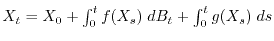
of the objects. The most important continuous time stochastic process definitely is Brownian motion
 . Standard Brownian motion is a stochastic process which
satisfies
. Standard Brownian motion is a stochastic process which
satisfies  ,
, ![$\E[B_t]=0$](images/img155.png) ,
,
![$\Cov[B_s,B_t] = s$](images/img156.png) for
for  and
for any sequence of times,
and
for any sequence of times,
 , the increments
 are all independent random vectors with normal distribution. Brownian motion is a solution
of the stochastic differential equation
are all independent random vectors with normal distribution. Brownian motion is a solution
of the stochastic differential equation
 , where
  is called white noise. Because white noise is only defined as a generalized function and
is not a stochastic process by itself, this stochastic differential
equation has to be understood in its integrated form
is called white noise. Because white noise is only defined as a generalized function and
is not a stochastic process by itself, this stochastic differential
equation has to be understood in its integrated form
 .
.
More generally, a solution to a stochastic differential equation
 is defined as the solution to the integral equation
 . Stochastic differential equations
can be defined in different ways. The expression
. Stochastic differential equations
can be defined in different ways. The expression
 can either be defined as an Ito integral, which leads to
martingale solutions, or the Stratonovich integral, which has similar integration
rules than classical differentiation equations. Examples of stochastic differential equations are
can either be defined as an Ito integral, which leads to
martingale solutions, or the Stratonovich integral, which has similar integration
rules than classical differentiation equations. Examples of stochastic differential equations are
 which has the solution
 . Or
. Or
 which has as the solution the process
 . The key tool to solve stochastic differential equations is Ito's
formula
. The key tool to solve stochastic differential equations is Ito's
formula
 ,
which is the stochastic analog of the fundamental theorem of calculus.
Solutions to stochastic differential equations are examples of Markov processes which show diffusion.
Especially, the solutions can be used to solve classical partial differential equations like the
Dirichlet problem
,
which is the stochastic analog of the fundamental theorem of calculus.
Solutions to stochastic differential equations are examples of Markov processes which show diffusion.
Especially, the solutions can be used to solve classical partial differential equations like the
Dirichlet problem  in a bounded domain
  with
with  on the boundary
  . One can
get the solution by computing the expectation of at the end points of Brownian motion starting at
and ending at the boundary
. One can
get the solution by computing the expectation of at the end points of Brownian motion starting at
and ending at the boundary
![$u = \E_x[f(B_T)]$](images/img175.png) . On a discrete graph, if Brownian motion is
replaced by random walk, the same formula holds too. Stochastic calculus is also useful to interpret quantum
mechanics as a diffusion processes [2,1] or as a tool to compute solutions
to quantum mechanical problems using Feynman-Kac formulas.
. On a discrete graph, if Brownian motion is
replaced by random walk, the same formula holds too. Stochastic calculus is also useful to interpret quantum
mechanics as a diffusion processes [2,1] or as a tool to compute solutions
to quantum mechanical problems using Feynman-Kac formulas.
Some features of stochastic process can be described using the language of Markov operators  ,
which are positive and expectation-preserving transformations on . Examples of such
operators are Perron-Frobenius operators
,
which are positive and expectation-preserving transformations on . Examples of such
operators are Perron-Frobenius operators  for a measure preserving transformation
 defining a discrete time evolution or stochastic matrices describing a random walk on a finite graph.
Markov operators can be defined by transition probability functions which are measure-valued
random variables. The interpretation is that from a given point , there are different possibilities
to go to. A transition probability measure
defining a discrete time evolution or stochastic matrices describing a random walk on a finite graph.
Markov operators can be defined by transition probability functions which are measure-valued
random variables. The interpretation is that from a given point , there are different possibilities
to go to. A transition probability measure
 gives the distribution of the target.
The relation with Markov operators is assured by the Chapman-Kolmogorov equation
gives the distribution of the target.
The relation with Markov operators is assured by the Chapman-Kolmogorov equation
 .
Markov processes can be obtained from random transformations, random walks or
by stochastic differential equations. In the case of a finite or countable target space
.
Markov processes can be obtained from random transformations, random walks or
by stochastic differential equations. In the case of a finite or countable target space  ,
one obtains Markov chains which can be described by probability matrices , which
are the simplest Markov operators. For Markov operators, there is an arrow of time: the relative entropy
with respect to a background measure is non-increasing. Markov processes often are attracted by fixed
points of the Markov operator. Such fixed points are called stationary states.
They describe equilibria and often they are measures with maximal entropy.
An example is the Markov operator , which assigns to a probability density
,
one obtains Markov chains which can be described by probability matrices , which
are the simplest Markov operators. For Markov operators, there is an arrow of time: the relative entropy
with respect to a background measure is non-increasing. Markov processes often are attracted by fixed
points of the Markov operator. Such fixed points are called stationary states.
They describe equilibria and often they are measures with maximal entropy.
An example is the Markov operator , which assigns to a probability density  the
probability density of
the
probability density of
 where
where
 is the random variable
  normalized so that it has mean and variance .
For the initial function
normalized so that it has mean and variance .
For the initial function  , the function
  is the distribution of
  the normalized sum of
  IID random variables
  . This Markov operator has a unique
equilibrium point, the standard normal distribution. It has maximal entropy among all distributions
on the real line with variance and mean . The central limit theorem tells that the
Markov operator has the normal distribution as a unique attracting fixed point if one takes
the weaker topology of convergence in distribution on . This works in other situations too.
For circle-valued random variables for example, the uniform distribution maximizes entropy. It is
not surprising therefore, that there is a central limit theorem for circle-valued random variables
with the uniform distribution as the limiting distribution.
. This Markov operator has a unique
equilibrium point, the standard normal distribution. It has maximal entropy among all distributions
on the real line with variance and mean . The central limit theorem tells that the
Markov operator has the normal distribution as a unique attracting fixed point if one takes
the weaker topology of convergence in distribution on . This works in other situations too.
For circle-valued random variables for example, the uniform distribution maximizes entropy. It is
not surprising therefore, that there is a central limit theorem for circle-valued random variables
with the uniform distribution as the limiting distribution.
In the same way as mathematics reaches out into other scientific areas, probability theory has
connections with many other branches of mathematics.
The last chapter of these notes give some examples. The section on percolation
shows how probability theory can help to understand critical phenomena.
In solid state physics, one considers
operator-valued random variables.
The spectrum of random operators are random objects too. One is interested
what happens with probability one. Localization is the
phenomenon in solid state physics that sufficiently
random operators often have pure point spectrum.
The section on estimation theory gives a glimpse of what mathematical statistics
is about. In statistics one often does not know the probability space itself so that one has to make a
statistical model and look at a parameterization of probability spaces. The goal is to give
maximum likelihood estimates for the parameters from data and to understand
how small the quadratic estimation error can be made.
A section on Vlasov dynamics shows how probability theory appears in problems of geometric evolution.
Vlasov dynamics is a generalization of the -body problem to the evolution of
of probability measures. One can look at the evolution of smooth measures or measures located on surfaces.
This deterministic stochastic system produces an evolution of densities which can form singularities
without doing harm to the formalism. It also defines the evolution of surfaces.
The section on moment problems is part of multivariate statistics. As for random variables,
random vectors can be described by their moments. Since moments define the law of the random variable,
the question arises how one can see from the moments, whether we have a continuous random variable.
The section of random maps is an other part of dynamical systems theory. Randomized versions of diffeomorphisms
can be considered idealization of their undisturbed versions. They often can be understood better than their
deterministic versions. For example, many random diffeomorphisms have only finitely many ergodic components.
In the section in circular random variables, we see that the Mises distribution has extremal
entropy among all circle-valued random variables with given circular mean and variance. There is also
a central limit theorem on the circle: the sum of IID circular random variables converges in law to the
uniform distribution. We then look at a problem in the geometry of numbers: how many lattice points
are there in a neighborhood of the graph of one-dimensional Brownian motion? The analysis of this problem
needs a law of large numbers for independent random variables with uniform distribution on ![$[0,1]$](images/img191.png) :
for
:
for
 , and
, and
![$A_n=[0,1/n^{\delta}]$](images/img193.png) one has
one has
 .
Probability theory also matters in complexity theory as a section on arithmetic random variables
shows. It turns out that random variables like
.
Probability theory also matters in complexity theory as a section on arithmetic random variables
shows. It turns out that random variables like  ,
,
 defined
on finite probability spaces become independent in the limit . Such considerations matter
in complexity theory: arithmetic functions defined on large but finite sets behave very much like
random functions. This is reflected by the fact that the inverse of arithmetic functions is in general
difficult to compute and belong to the complexity class of NP. Indeed, if one could invert arithmetic
functions easily, one could solve problems like factoring integers fast.
A short section on Diophantine equations indicates how the distribution of random variables can shed
light on the solution of Diophantine equations. Finally, we look
at a topic in harmonic analysis which was initiated by Norbert Wiener.
It deals with the relation of the characteristic function
defined
on finite probability spaces become independent in the limit . Such considerations matter
in complexity theory: arithmetic functions defined on large but finite sets behave very much like
random functions. This is reflected by the fact that the inverse of arithmetic functions is in general
difficult to compute and belong to the complexity class of NP. Indeed, if one could invert arithmetic
functions easily, one could solve problems like factoring integers fast.
A short section on Diophantine equations indicates how the distribution of random variables can shed
light on the solution of Diophantine equations. Finally, we look
at a topic in harmonic analysis which was initiated by Norbert Wiener.
It deals with the relation of the characteristic function  and the
continuity properties of the random variable .
and the
continuity properties of the random variable .
Colloquial language is not always precise enough to tackle problems
in probability theory. Paradoxes appear, when definitions allow
different interpretations. Ambiguous language can lead to wrong conclusions
or contradicting solutions. To illustrate this, we mention a few problems.
The following four examples should serve as a motivation to introduce
probability theory on a rigorous mathematical footing.
1) Bertrand's paradox (Bertrand 1889)
We throw at random lines onto the unit disc.
What is the probability that the line intersects the disc with
a length  , the length of the inscribed equilateral
triangle?
, the length of the inscribed equilateral
triangle?
First answer: take an arbitrary point on the boundary of the disc. The set of
all lines through that point are parameterized by an angle  . In
order that the chord is longer than
. In
order that the chord is longer than  , the line has to lie within
a sector of
, the line has to lie within
a sector of  within a range of
  . The probability is .
Second answer: take all lines perpendicular to a fixed diameter.
The chord is longer than if the point of intersection
lies on the middle half of the diameter. The probability is  .
.
Third answer: if the midpoints of the chords lie in a
disc of radius , the chord
is longer than . Because the disc has a radius which is
half the radius of the unit disc, the probability is  .
.
Like most paradoxes in mathematics, a part of the question in Bertrand's problem
is not well defined. Here it is the term "random line". The solution of the
paradox lies in the fact that the three answers depend
on the chosen probability distribution. There are several "natural"
distributions. The actual answer depends on how the experiment is performed.
2) Petersburg paradox (D.Bernoulli, 1738)
In the Petersburg casino, you pay an entrance fee  and you
get the prize
and you
get the prize  , where is the number of times, the casino flips
a coin until "head" appears. For example, if the sequence
of coin experiments would give "tail, tail, tail, head", you would
win
, where is the number of times, the casino flips
a coin until "head" appears. For example, if the sequence
of coin experiments would give "tail, tail, tail, head", you would
win  , the win minus the entrance fee. Fair would be an
entrance fee which is equal to the expectation of the win, which is
, the win minus the entrance fee. Fair would be an
entrance fee which is equal to the expectation of the win, which is
![\begin{displaymath}\sum_{k=1}^{\infty} 2^k \Prob[T=k] = \sum_{k=1}^{\infty} 1 = \infty \; . \end{displaymath}](images/img208.png)
The paradox is that nobody would agree to pay even an entrance fee  .
.
The problem with this casino is that it is not quite clear, what is "fair".
For example, the situation  is so improbable that it never occurs in
the life-time of a person. Therefore, for any practical reason, one has not
to worry about large values of . This, as well as the finiteness of money
resources is the reason, why casinos do not have to worry about the following
bullet proof martingale strategy
in roulette: bet dollars on red. If you win, stop, if you lose,
bet
is so improbable that it never occurs in
the life-time of a person. Therefore, for any practical reason, one has not
to worry about large values of . This, as well as the finiteness of money
resources is the reason, why casinos do not have to worry about the following
bullet proof martingale strategy
in roulette: bet dollars on red. If you win, stop, if you lose,
bet  dollars on red. If you win, stop. If you lose, bet
  dollars
on red. Keep doubling the bet. Eventually after steps, red will occur
and you will win
dollars
on red. Keep doubling the bet. Eventually after steps, red will occur
and you will win
 dollars. This example
motivates the concept of martingales.
Theorem (
dollars. This example
motivates the concept of martingales.
Theorem (![[*]](images//usr/share/latex2html/icons/crossref.png) ) or proposition ()
will shed some light on this. Back to the Petersburg paradox. How does one
resolve it? What would be a reasonable entrance fee in
"real life"? Bernoulli proposed to replace the expectation
) or proposition ()
will shed some light on this. Back to the Petersburg paradox. How does one
resolve it? What would be a reasonable entrance fee in
"real life"? Bernoulli proposed to replace the expectation ![$\E[G]$](images/img214.png) of
the profit
of
the profit  with the expectation
![$(\E[\sqrt{G}])^2$](images/img216.png) , where
, where
 is called a utility function.
This would lead to a fair entrance
is called a utility function.
This would lead to a fair entrance
![\begin{displaymath}(\E[\sqrt{G}])^2=(\sum_{k=1}^{\infty} 2^{k/2} 2^{-k})^2
= \frac{1}{(\sqrt{2}-1)^2} \sim 5.828... \; . \end{displaymath}](images/img218.png)
It is not so clear if that is a way out of the paradox because for
any proposed utility function  , one can modify the casino rule
so that the paradox reappears: pay
, one can modify the casino rule
so that the paradox reappears: pay  if the utility
function
if the utility
function  or pay
  dollars, if the utility function
is
dollars, if the utility function
is
 . Such reasoning plays a role in economics and social
sciences.
. Such reasoning plays a role in economics and social
sciences.
The picture to the right shows the average profit development during a
typical tournament of 4000 Petersburg games. After these 4000 games, the player
would have lost about 10 thousand dollars, when paying a 10 dollar entrance fee
each game. The player would have to play a very, very long time to catch up. Mathematically,
the player will do so and have a profit in the long run, but it is unlikely that it will
happen in his or her life time.
3) The three door problem (1991)
Suppose you're on a game show and you are given a choice of three
doors. Behind one door is a car and behind the others are goats. You
pick a door-say No. 1 - and the host, who knows what's behind the doors,
opens another door-say, No. 3-which has a goat. (In all games, he
opens a door to reveal a goat). He then says to you, "Do you want to
pick door No. 2?" (In all games he always offers an option to switch).
Is it to your advantage to switch your choice?
The problem is also called "Monty Hall problem" and
was discussed by Marilyn vos Savant in a "Parade" column
in 1991 and provoked a big controversy. (See [3] for
pointers and similar examples.)
The problem is that intuitive argumentation can easily lead to the conclusion
that it does not matter whether to change the door or not. Switching the door
doubles the chances to win:
No switching: you choose a door and win with probability 1/3. The opening
of the host does not affect any more your choice.
Switching: when choosing the door with the car, you loose since you switch.
If you choose a door with a goat. The host opens the other door with the goat
and you win. There are two such cases, where you win.
The probability to win is 2/3.
4) The Banach-Tarski paradox (1924)
It is possible to cut the standard unit ball
 into 5 disjoint pieces
 and rotate and translate
the pieces with transformations
and rotate and translate
the pieces with transformations  so that
 and
and
 is a second unit ball
 and all the transformed sets again
don't intersect.
and all the transformed sets again
don't intersect.
While this example of Banach-Tarski is spectacular, the existence of bounded subsets of the circle
for which one can not assign a translational invariant probability ![$\Prob[A]$](images/img230.png) can already be achieved
in one dimension.
The Italian mathematician Giuseppe Vitali gave in 1905 the following example: define an
equivalence relation on the circle
can already be achieved
in one dimension.
The Italian mathematician Giuseppe Vitali gave in 1905 the following example: define an
equivalence relation on the circle
 by saying that two angles are equivalent
 if
if  is a rational
angle. Let be a subset in the circle which contains exactly one number from each equivalence
class. The axiom of choice assures the existence of . If
is a rational
angle. Let be a subset in the circle which contains exactly one number from each equivalence
class. The axiom of choice assures the existence of . If
 is a enumeration of the
set of rational angles in the circle, then the sets
is a enumeration of the
set of rational angles in the circle, then the sets  are pairwise disjoint and satisfy
 . If we could assign a translational invariant probability
![$\Prob[A_i]$](images/img237.png) to , then the basic rules of probability would give
to , then the basic rules of probability would give
![\begin{displaymath}1 = \Prob[\TT] = \Prob[ \bigcup_{i=1}^{\infty} A_i ] = \sum_{i=1}^{\infty} \Prob[A_i] = \sum_{i=1}^{\infty} p \; . \end{displaymath}](images/img238.png)
But there is no real number
![$p=\Prob[A]=\Prob[A_i]$](images/img239.png) which makes this possible.
which makes this possible.
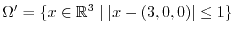
Both the Banach-Tarski as well as Vitalis result shows that one can not hope
to define a probability space on the algebra of all subsets of the unit ball or
the unit circle such that the probability measure is translational and rotational invariant.
The natural concepts of "length" or "volume", which are rotational and translational invariant
only makes sense for a smaller algebra. This will lead to the notion of -algebra.
In the context of topological spaces like Euclidean spaces, it leads to
Borel -algebras, algebras of sets generated by the compact sets of the
topological space. This language will be developed in the next chapter.
Probability theory is a central topic in mathematics. There are close
relations and intersections with other fields like computer science,
ergodic theory and dynamical systems, cryptology, game theory,
analysis, partial differential equation, mathematical physics,
economical sciences, statistical mechanics and even number theory.
As a motivation, we give some problems and topics which
can be treated with probabilistic methods.
1) Random walks:
(statistical mechanics, gambling, stock markets, quantum field theory).
Assume you walk through a lattice. At each vertex, you choose a direction
at random. What is the probability that you return back to your starting point?
Polya's theorem () says that in two
dimensions, a random walker almost
certainly returns to the origin arbitrarily often, while in three dimensions,
the walker with probability only returns a finite number of times and then
escapes for ever.
A random walk in one dimensions displayed as a graph 
2) Percolation problems
(model of a porous medium, statistical mechanics, critical phenomena).
Each bond of a rectangular lattice in the plane is connected with probability  and disconnected with probability
  . Two lattice points
  in the lattice are
in the same cluster, if there is a path from to
in the lattice are
in the same cluster, if there is a path from to  .
One says that "percolation occurs" if there is
a positive probability that an infinite cluster appears.
One problem is to find the critical probability
.
One says that "percolation occurs" if there is
a positive probability that an infinite cluster appears.
One problem is to find the critical probability  , the
infimum of all , for which percolation occurs. The problem can be
extended to situations, where the switch probabilities are not
independent to each other. Some random variables like the size of the largest
cluster are of interest near the critical probability .
, the
infimum of all , for which percolation occurs. The problem can be
extended to situations, where the switch probabilities are not
independent to each other. Some random variables like the size of the largest
cluster are of interest near the critical probability .
A variant of bond percolation is site percolation where the nodes of the lattice
are switched on with probability .
Generalized percolation problems are obtained, when the independence of the
individual nodes is relaxed. A class of such dependent percolation problems can be obtained by
choosing two irrational numbers  like
like
 and
and
 and switching the node
  on if
on if
 . The
probability of switching a node on is again , but the random variables
. The
probability of switching a node on is again , but the random variables
are no more independent.
Even more general percolation problems are obtained, if also the distribution of the
random variables  can depend on the position .
3) Random Schrödinger operators.
(quantum mechanics, functional analysis, disordered systems, solid state physics)
Consider the linear map
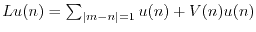 on the space of
sequences
on the space of
sequences
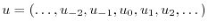 .
We assume that
.
We assume that  takes random values in
  . The function
  is called
the potential. The problem is to determine the spectrum or spectral type of the infinite
matrix
is called
the potential. The problem is to determine the spectrum or spectral type of the infinite
matrix  on the Hilbert space
 of all sequences
  with finite
 . The
operator is the Hamiltonian of an electron in a one-dimensional disordered crystal.
The spectral properties of have a relation with the conductivity properties
of the crystal. Of special interest is the situation, where the values are all
independent random variables.
It turns out that if are IID random variables with a continuous distribution,
there are many eigenvalues for the infinite dimensional matrix - at least with
probability . This phenomenon is called localization.
. The
operator is the Hamiltonian of an electron in a one-dimensional disordered crystal.
The spectral properties of have a relation with the conductivity properties
of the crystal. Of special interest is the situation, where the values are all
independent random variables.
It turns out that if are IID random variables with a continuous distribution,
there are many eigenvalues for the infinite dimensional matrix - at least with
probability . This phenomenon is called localization.
A wave
 evolving in a random potential at
 . Shown are both the potential
  and the wave
  A wave
evolving in a random potential at
A wave
evolving in a random potential at
 . Shown are both the potential and the wave
  A wave
evolving in a random potential at
A wave
evolving in a random potential at
 . Shown are both the potential and the wave
More general operators are obtained by allowing to be random variables with the
same distribution but where one does not persist on independence any more. A well studied
example is the almost Mathieu operator, where
 and for which
  is irrational.
4) Classical dynamical systems
(celestial mechanics, fluid dynamics, mechanics, population models)
The study of deterministic dynamical systems like the logistic map
 on the interval or the three body problem in
celestial mechanics has shown that such systems or subsets of it can behave like random systems.
Many effects can be described by ergodic theory, which
can be seen as a brother of probability theory. Many results
in probability theory generalize to the more general setup of
ergodic theory. An example is Birkhoff's ergodic theorem
which generalizes the law of large numbers.
on the interval or the three body problem in
celestial mechanics has shown that such systems or subsets of it can behave like random systems.
Many effects can be described by ergodic theory, which
can be seen as a brother of probability theory. Many results
in probability theory generalize to the more general setup of
ergodic theory. An example is Birkhoff's ergodic theorem
which generalizes the law of large numbers.
Iterating the logistic map
on produces independent
random variables. The invariant measure is continuous.
The simple mechanical system of a double pendulum exhibits complicated dynamics.
The differential equation defines a measure preserving flow  on a probability
A short time evolution of the Newtonian three body problem. There are
energies and subsets of the energy surface which are invariant and on which there is
an invariant probability measure.
on a probability
A short time evolution of the Newtonian three body problem. There are
energies and subsets of the energy surface which are invariant and on which there is
an invariant probability measure.
Given a dynamical system given by a map or a flow on a subset of some Euclidean space,
one obtains for every invariant probability measure a probability space
.
An observed quantity like a coordinate of an individual particle is a random variable and defines
a stochastic process
 . For many dynamical systems including also some
3 body problems, there are invariant measures and observables for which are IID random variables.
Probability theory is therefore intrinsically relevant also in classical dynamical systems.
. For many dynamical systems including also some
3 body problems, there are invariant measures and observables for which are IID random variables.
Probability theory is therefore intrinsically relevant also in classical dynamical systems.
5) Cryptology.
(computer science, coding theory, data encryption)
Coding theory deals with the mathematics of encrypting codes or deals with the
design of error correcting codes. Both aspects of coding theory have important
applications. A good code can repair loss of information due to bad channels and
hide the information in an encrypted way. While many aspects of coding theory are
based in discrete mathematics, number theory, algebra and algebraic geometry, there
are probabilistic and combinatorial aspects to the problem. We illustrate this
with the example of a public key encryption algorithm whose security is based on
the fact that it is hard to factor a large integer
 into its prime factors
  but easy to verify that are factors, if
one knows them. The number
but easy to verify that are factors, if
one knows them. The number  can be public but only the
person, who knows the factors can read the message. Assume, we want to crack
the code and find the factors and
can be public but only the
person, who knows the factors can read the message. Assume, we want to crack
the code and find the factors and  .
.
The simplest method is to try to find the factors by trial and error but this is
impractical already if has 50 digits. We would have to search through  numbers to find the factor . This corresponds to probe 100 million times every second over a
time span of 15 billion years. There are better methods known and we want to illustrate one
of them now: assume we want to find the factors of
numbers to find the factor . This corresponds to probe 100 million times every second over a
time span of 15 billion years. There are better methods known and we want to illustrate one
of them now: assume we want to find the factors of
 .
The method goes as follows: start with an integer
.
The method goes as follows: start with an integer  and iterate the
quadratic map
and iterate the
quadratic map
 on
on
 . If we assume the
numbers
. If we assume the
numbers
 to be random, how many such numbers do we have to
generate, until two of them are the same modulo one of the prime factors ?
The answer is surprisingly small and based on the birthday paradox:
the probability that in a group of 23 students, two of them have the
same birthday is larger than : the probability of the event that we have
no birthday match is
to be random, how many such numbers do we have to
generate, until two of them are the same modulo one of the prime factors ?
The answer is surprisingly small and based on the birthday paradox:
the probability that in a group of 23 students, two of them have the
same birthday is larger than : the probability of the event that we have
no birthday match is
 , so that the probability of
a birthday match is
, so that the probability of
a birthday match is
 . This is larger than .
If we apply this thinking to the sequence of numbers generated by the
pseudo random number generator , then we expect to have a chance of for finding
a match modulo in
. This is larger than .
If we apply this thinking to the sequence of numbers generated by the
pseudo random number generator , then we expect to have a chance of for finding
a match modulo in  iterations. Because
 , we have to try
 numbers, to get a factor: if
  and
and  are the same modulo ,
then
are the same modulo ,
then
 produces the factor of . In the above
example of the 46 digit number , there is a prime factor
produces the factor of . In the above
example of the 46 digit number , there is a prime factor  . The
Pollard algorithm finds this factor with probability in
. The
Pollard algorithm finds this factor with probability in  steps.
This is an estimate only which gives the order of magnitude. With the above ,
if we start with
steps.
This is an estimate only which gives the order of magnitude. With the above ,
if we start with  and take
  , then we have a match
 .
It can be found very fast.
.
It can be found very fast.
This probabilistic argument would give a rigorous probabilistic estimate if we would pick truly
random numbers. The algorithm of course generates such numbers in a deterministic way
and they are not truly random. The generator is called a pseudo random number generator.
It produces numbers which are random in the sense that many statistical tests can not
distinguish them from true random numbers. Actually, many random number generators built into
computer operating systems and programming languages are pseudo random number generators.
Probabilistic thinking is often involved in designing, investigating and
attacking data encryption codes or random number generators.
6) Numerical methods.
(integration, Monte Carlo experiments, algorithms)
In applied situations, it is often very difficult to find integrals
directly. This happens for example in statistical mechanics or
quantum electrodynamics, where one wants to find integrals in spaces
with a large number of dimensions. One can nevertheless compute
numerical values using Monte Carlo Methods with a manageable
amount of effort. Limit theorems assure that these numerical values
are reasonable. Let us illustrate this with a very simple but famous example,
the Buffon needle problem.
A stick of length 2 is thrown onto the plane filled with
parallel lines, all of which are distance  apart. If the center of the stick
falls within distance of a line, then the interval of angles
leading to an intersection with a grid line has length
apart. If the center of the stick
falls within distance of a line, then the interval of angles
leading to an intersection with a grid line has length
 among a possible range of angles
 ![$[0,\pi]$](images/img302.png) .
The probability of hitting a line is therefore
.
The probability of hitting a line is therefore
 .
This leads to a Monte Carlo method to compute
.
This leads to a Monte Carlo method to compute  . Just throw randomly sticks onto
the plane and count the number
. Just throw randomly sticks onto
the plane and count the number  of times, it hits a line. The
number
of times, it hits a line. The
number  is an approximation of . This is of course not an effective way
to compute but it illustrates the principle.
is an approximation of . This is of course not an effective way
to compute but it illustrates the principle.
The Buffon needle problem is a Monte Carlo method to
compute . By counting the number of hits in a sequence
of experiments, one can get random approximations of .
The law of large numbers assures that the approximations will
converge to the expected limit. All Monte Carlo computations are theoretically
based on limit theorems.
