A Lecture on Partial Differential Equations

1. Partial Differential Equations

An equation for an unknown function f involving partial derivatives of f is called a partial differential equation. Essentially all fundamental laws of nature are partial differential equations as they combine various rate of changes. We are affected by partial differential equations on a daily basis: light and sound propagates according to the wave equation which is a consequence of the Maxwell equations, the fabric of space and time are described by the Einstein equations which tells how mass affects distance. The heat equation describes diffusion, the propagation of energy or is used in smoothing procedures of computer vision. Laws like the Navier-Stokes equations govern the motion of fluids or gases, the currents in the ocean or the winds in the atmosphere. On a fundamental level, the laws of particle motion is not given by ordinary differential equations like the Newton equations which describe the motion of planets but by partial differential equations, the Schrödinger equation in particular. In quantum mechanics, a physical configuration is modeled by a complex-valued function like the wave function of a particle or the wave function of the universe. Its time evolution is the Schröodinger or Dirac equation. Unexpectedly, partial differential equations also appear in finance. The infamous Black-Scholes equation for example relates the prices of options with stock prices. In the course-wide introduction lecture of this Math 21a course on September 3, 2019, one slide illustrated the front page of a book of Ian Stewart "In Pursuit of the Unknown, 17 equations that changed the world". You see the book cover again on the left. At the end of the present lecture we want to see in a worksheet whether we can identify a few laws. The goal of this lecture is to get you exposed to partial differential equations. You should also know a few partial differential equations personally. They should be your friends in the sense that you know what they do and for what adventure you can join them. By the way, you already know one partial differential equation: it is the Clairaut equation fxy = fyx from last lecture. It is a partial differential equation because it involves an unknown function f and involves partial derivatives with respect to x and y. This equation appears maybe a bit silly like the equation x = x, which is satisfied for all x. We have seen in the last lecture that the Clairaut equation is satisfied for all functions which we can continuously differentiate twice.

2. The Transport Equation

The transport equation ft = fx for the unknown function f(t,x) describes transport. It is also called advection equation. The rule is a basic model for signal processing and is of the simplest partial differential equations which exist. The picture to the left (click on it to see it larger) explains what is going on. We are given a signal f(0,x) at time t=0. The equation tells how that signal looks like at a later time like t=1. If you look at the partial differential equation, then it relates the slope of the signal fx with the rate of change in time. If the x-slope is negative, then the function is pushed down there. This is indicated with the green arrows in the picture. If the slope is positive, the function is pushed up. P.S. Here is something for those of you who have seen Taylor series in Math 1b: given any nice function g of one variable, the function f(t,x) = g(x+t) satisfies the transport equation. Check this by taking the derivative with respect to t and the derivative with respect to x! We can now write the transport equation as ft = D f, where D means taking the derivative. You might also remember what the solution of the differential equation f' = a f was. It is f(t) = eat f(0) = (1 + a t + a2 t2/2 + .... ). If we replace a with D, then this becomes f(t) = e D t f = f(0) + t D f(0) + t2 D2/2 f(0) + ... = f(0) + t f'(0) + t^2 f''(0)/2 + ..., which is the Taylor series of the function. We say, that the derivative generates translation. Applying that to the function g gives g(x+t)= f(x) + t D f(x) t + t^2 f''(0)/2 + ..., which is Taylor's theorem. The transport equation can also be seen as the Schrödinger equation i h d/dt ψ(t) = P ψ for the momentum operator P = iD in quantum mechanics where the constant h is the Planck constant. Isn't that cool? The motion of a free particle without being exposed to an external force is just uniform translation. This is one of Newton's laws who formulated it as ``Every object in a state of uniform motion will remain in that state of motion unless an external force acts on it." The language of quantum mechanics describes this in terms of functions and this is the Taylor theorem. Using a Taylor series with a few terms already gives a good approximation of the real situation. In quantum mechanics, this idea is pushed much further and leads to Feynman path integrals describing the interaction of particles. Some Schrödinger equation animations from 2001, the C program has computed also the animation to the right. I wrote that program shortly after writing this paper on quantum dynamics.

3. The Heat Equation

The heat equation ft = fxx for the unknown function f(t,x) describes the propagation of heat. It is also called diffusion equation. Essentially anything which spreads randomly can be modeled by some sort of heat equation. The function f(t,x) can for example describe the concentration of a chemical as a function of time t and position x. What happens with the substances is that they diffuse, mostly due to thermal motion. If we write the right hand side in a discrete form by using h fx(t,x) = f(x+h,t)-f(x,t), then h2 fxx(t,x-h) = f(t,x+h)-2f(t,x)+f(t,x-h) which combines concentration levels of the neighbors. It is positive if f(x) is smaller than the average of f(t,x+h) and f(t,x-h). Let us look at it geometrically. The second derivative fxx(t,x) is concavity. If the function is concave up in the x direction, then fxx(t,x) is positive. The heat equation then tells that ft is positive there and the function should increase in time there. On the other hand, if the function is concave down in the x direction, then fxx(t,x) is negative and the function decreases there. We see that mountain hills get pushed down and valleys get filled up. Applying the heat equation is a sort of ``erosion". When applying the heat equation to a picture, then the picture gets blurred out. The heat equation is essential also in probability theory as probability density functions describing a random process like a random walk move according to diffusion equations. The theory of stochastic processes is essentially the theory of partial differential equations. This applies also to discrete processes which are described by partial difference equations, the discrete analogue of partial differential equations. P.S. The heat equation is used in many other set-ups. Whenever one has a ``Laplacian" L on a space, then ft = L f is a heat equation. This applies also in discrete worlds like networks on which one can define Laplacians. One can look at partial differential equations on graphs for example. See this HCRP project which led to a thesis of Annie Rak in applied mathematics. The heat equation is one of the most fundamental principles in mathematics. It is used to prove theorems. The proof that any 3-dimensional space on which every loop can be contracted to a point is a 3-dimensional sphere was done using the Ricci flow which is a heat equation.

4. The Wave Equation

The wave equation ftt = fxx for the unknown function f(t,x) describes the motion of a string. It also can model water waves, light or sound. As we have now a second derivative in time, the right hand side should be interpreted as the force acting on the string or water surface. If the wave is high, then it is pushed down. However unlike for the heat equation where things converge to zero, the height energy is transformed into kinetic energy and even if f(0,x) can be zero, there can be an initial velocity ft(0,x) in the string. Taking a string and plucking it is the case when we start with an initial position without initial velocity. If we hit the string like what the hammer of a piano does, then we give it an initial velocity. The wave motion is less intuitive as we have also velocity hidden in the string. We will make some experiments which explains this. For now, let us just look at the d'Alembert solution. Given two functions g(x) and h(x) of one variable, then f(t,x) = g(x+t) + h(x-t) solves the wave equation. For example if g(x) = x3 and h(x) = sin(5x), then we have the function f(t,x) = (x+t)3 + sin(5(x-t)). You can check that this solves the heat equation. If we take f(t,x) = [g(x+t) + g(x-t)]/2 then this function solves the wave equation with the initial condition f(0,x)=g(x) and ft(0,x) = 0. It is the situation when we throw a rock in a narrow water channel. There are two signals which travel to both sides. Actually both satisfy the transport equation. Similarly, you can see that f(t,x) = [h(x+t) - h(x-t)]/2 has the property that f(0,x)=0 and ft(0,x) = h(x). It should be obvious that because light and sound is described by the wave equation that this is an important partial differential equation. Nikola Tesla once said: ``If you want to find the secrets of the Universe, think in terms of energy, frequency and vibration.".

5. The Burgers Equation

The Burgers equation is the partial differential equation ft = f fx As it can describe waves reaching a beach, it is the ``surfers equation". Unlike the other equations considered so far, the equation is a nonlinear equation. If we multiply f a constant 2 for example, then the right hand side is multiplied by 4 and the left by 2. Let us first look at the transport equation ft = c fx again, but let us now introduce a constant c. This equation has solutions g(x+ct) so that c can be interpreted as the speed of the signal. now, in the case of the Burgers equation, the speed c depends on the height f of the wave. A higher wave will travel faster than a lower one. This has the consequence that the waves tend to become steeper and the fall over. This happens near the beach.

The Burgers equation can be generalized. First of all, one can add a viscosity term μ fxx which adds a diffusion. Then one can add more forces due to pressure and possible external forces. These are complicated equations. One has to determine the pressure from an additional partial differential equation. To the right, we see a scene from the movie ``Gifted" (see a few clips from gifted here in larger format), in which the Millenium problem about Navier Stokes appears.

5. The Laplace Equation

The Laplace equation fxx + fyy = 0 is not a time evolution equation. The two variables x and y should both be seen as space variables. The equation tells that the function is ``harmonic", meaning that f describes some sort of equilibrium. One can look at this equation also in the case when f(x,y) is kept fixed on the boundary of some region. One calls this then a Dirichlet problem. Related to the Laplace equation is the problem to find solutions of the equation fxx + fyy = λ f, where f is a function in a region but fixed on the boundary. The frequencies λ for which we have a solution are called ``resonance frequencies of the region". These are the frequencies one can hear. It does not have to be a drum, it can be a violine. The solutions f(x,y) can be seen by exciting the plate in that frequency and then put some powder on it. The powder particles then will accumulate at the level curves where f(x,y) = 0. These contour curves are called Chladni figures. We will try to make some experiments in class. P.S. Harmonic functions play an important role everywhere in mathematics, for example when calculus is done in the complex. Let us look for example at the function g(z) = z3 in the complex, where z=x+i y is a complex number. You might not have seen complex numbers but i stands for the square root of -1. One can calculate with complex numbers like with other numbers but just has to keep in mind that i2 can be replaced by -1. For example, with g(z) = (x+i y)3 then this is x3 + 3 i x2 y - 3 x y2 - i y3. This is the complex number with real part u(x,y) = x3 - 3 x y2 and imaginary part v(x,y) = 3 x2 y - y3. As you can check, both of these functions u(x,y) and v(x,y) satisfy the Laplace equation.

The Laplace equation can also be studied on graphs. See this video:

6. Dangerous Ideas

A ``dangerous idea seminar" framework has been a MIT tradition for decades, where the speaker has to structure the talk around five questions based on Fear, Joy, Mom, Cool, New. The questions can be adapted also to each lecture. Lets do that: 1. Why should I fear the topic? Partial differential equation ideas are used in any technology, this includes face recognition, building weapons etc. But this can be said about essentially any science. But you know what is probably the most scary thing about PDE's: the topic is not easy! It is a quite technical area of mathematics. Also when studying the topic with a computer, one has to deal with complicated numerical frame works. One has to work hard in order to make numerical approximations which are robust and for which the numerical solution is close to the actual solution one sees when one makes the experiment. 2. Why should I rejoice it to be done? Partial differential equations are the fabric we are made of. Understanding the Schrödinger equation allows us to understand elementary particles. Just an example. If one looks at the Energy operator L of a Hydrogen atom, then the structure of the eigenvalues describes the periodic system of elements. Partial differential equations are used to predict the weather, the paths of hurricanes, the impact of a tsunami, the flight of an aeroplane. They are used to understand complex stochastic processes. Partial differential equations appear everywhere in engineering, also in machine learning or statistics. A generalization of the transport is the gradient flow which is used to get good solutions to problems. As mentioned at the beginning, all fundamental laws in nature (classical mechanics can be described by variational problems leading to partial differential equations, the Euler equations, general relativity is described by the Einstein equations, gravitational waves emerging from a black hole merger recently measured out allows us to see what happened billions of years ago in an other part of the universe, diffusion equations can help to track the spreading of a virus or environmental disaster like an oil spill). 3. What should I tell my mom about it? Partial differential equations allows us to look into the future and allows us to take action in order to avoid difficult situations. Similarly as ordinary differential equations allow us to predict how far an asteroid zooms by the earth, we can build and use models to predict how the climate changes, we can take measures to soften the impact of a storm, or use it even for rather mundane things like how to make money (or lose some ...) on the stock market. 4. What is a cool discovery in that field? One of the fundamental results is the theorem of Cauchy-Kovalevski which assures a system of partial differential equations with analytic functions as coefficients has a unique solution. This is quite subtle, as analyticity is stronger than just smoothness. Analytic functions are functions which have a Taylor series which converges. 5. What is a recent discovery in the subject? 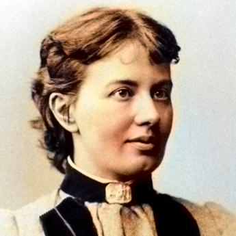A rather recent discovery is a result of Gregory Perelmann which tells that a simply connected bounded three dimensional space must be a three dimensional sphere. The theorem was proven using some sort of heat equation acting on a curvature functions. Given the space, the space is deformed by applying the heat flow. The flow smooths out the space, making it round. The limiting shape is then a sphere, like the bubbles seen in the lava lamp placed on the table during the lecture.

7. Mathematicians

Sofia Kowalevskaja (general PDE)	Augustine Cauchy (general PDE)	Johannes Martinus Burgers (Burgers eqn)
Pierre-Simon Laplace (Laplace eqn)	Jean d'Alembert (Wave eqn)	Joseph Fourier (Heat eqn)

Appendix: On this lecture