May 27, 2017: : here are some slides authored in the fall 2015 and spring 2016. There is
some addition as for the connection Laplacian, the Barycentric limit shows a
mass gap. Also on
the quantum calculus blog are some new doodles from how
to get a grip on the quantum plane. I decided to put the slightly updated slides on
the Barycentric limit story on youtube rather having it rotting and lost on the hard drive:
October 21, 2015:
Here are explicit "coordinate transformations" in the case d=6 to go from
Barycentric invariants, the eigenvectors of the 7x7 matrix AT
How does the explicit integer coordinate transformation look like in general?
Here is an other example: the basis change matrix which maps the Dehn-Sommerville
numbers to the Barycentric numbers. I don't see the formula for the matrix entries yet.
We know the Dehn-Sommerville numbers explicitly as we do know the eigenvectors of
the Barycentric matrix (the Barycentric characteristic numbers). So, in principle, we
could get "really messy" formulas for the basis change matrix.
October 15, 2015:
The language of graph theory is less familiar in the context of Barycentric refinement. While
the concept of simplicial complexes is more general, it is actually enough to look at graphs.
There are two point of views: one is to see a simplicial complex as an additional structure
on a set like a topological, measure an order or algebraic structure: a simplicial complex
is simply a subset of the set of subsets which is closed under forming subsets.
There is an other point of view, which is taken in geometric probability theory: given
a simplicial complex, one can look at the lattice generated by all simplicial sub complexes
and define so valuations. If the set of sub complexes form the vertex set of a graph, and if we form the
edge set as the set of pairs where one is contained in the other, then this defines a graph
which contains all the essential information about the complex. If the simplicial complex
was the Whitney of a graph, then the new graph is just the Barycentric refinement. In any
case, we see that it does not matter whether we start with a simplicial complex or a graph
when doing refinements. We always get already after one step to complexes which can be
described by graphs. So, when looking at Barycentric refinements, and especially when iterating
them, we have no reason to carry around the language of simplicial complexes.
Just start with a graph and define from it a new graph.
This is not only simpler, it also removes any possible confusion as Barycentric
refinement is usually considered in an Euclidean setting or for structures embedded in an
Euclidean space.
October 13, 2015:
Start with the spectrum {l(1),..,l(n)} of a graph, then there is no reason why
the logarithmic energy sum_(i not equal to j) -log|l(i)-l(j)| should be minimal when restricted to an interval
[0,max( spectrum(L))]. What happens in the one dimensional case is that under refinement, the spectrum
gets closer and closer to the minimal logarithmic point set energy. This follows from the spectral
measure convergence in one dimensions. To describe such a situation in the 2 or higher dimensional
case is more difficult as we don't know the nature of the support of the measure in the limit. But its
reasonable to think that the logarithmic energy of the spectral measures converges to the minimum once we
know the gaps in the spectrum. Unfortunately we have not even shown the existence of a single gap in the
spectrum.
October 12, 2015:
Is the limiting group indeed just the product of two dyadic groups of integers?
The presentation of the limiting group will no more be finite but isomorphic as a group.
Here is a simple example: the group Z4 can be generated
by one generator or by two. The group stays the same but the Cayley graph
changes and becomes triangular. The limiting group of the Barycentric refinement
has a countable set of generators and many relations. If we look at the limiting
random ergodic operator, then any representation as a matrix in some basis has
infinitely many entries in most rows and columns. This is obvious also from the
fact that the limiting Laplacian is an unbounded operator, unlike in one dimensions,
where it is a bounded Jacobi matrix. An example of an infinitely generated presented
group is Z with generators ak(x) = x+2^k which has the property that
the generators satisfy the relations ak^2 = a k+1. The Cayley graph
has now infinite vertex degree at each vertex and the corresponding Laplacian is unbounded.
The original Laplacian of Z is the free Jacobi matrix, the limiting Barycentric operator
in one dimensions. There are two ways to see more structure: one is ergodic theory as
discussed below (fixed point of a 2:1 integral extension map among dynamical systems), the other
is potential theory as the equilibrium measure on the spectrum [0,4] is the arc sin
distribution which is invariant under the quadratic map having the spectrum as Julia set.
One could experimentally check whether the density of states in the two dimensional case is
the equilibrium measure on the spectrum as a set, minimizing the logarithmic energy, the measure
which leads to logarithmic capacity.
October 11, 2015:
The Z2 dynamical system renormalization defines a refinement
of the grid, but we need other finitely presented groups to model
the Barycentric refinement. For d=2, we need 6 generators already
after one step. On each triangle, we have to renormalize
(S,T,R) -> (S',T',R',U',V',W').
We do that with four intervals. The first one belongs to the vertices,
the two next ones to edges and the final one to triangles.
First double S and T, form R.
Now define U as half of TS. Then define V,W. Now we have
6 transformations on the interval. An orbit of the so obtained
finitely presented group defines the Barycentric subdivision.
In the next refinement, we have to renormalize in each triangle
and get a group with 12 generators.
The generators can all be obtained from S,T and their refinements
but we need the new generators to define the graph structure and so
the Laplacian at each stage. The frame work of ergodic theory
has an advantage about inverse limit constructions
as there is a natural completeness built in already: taking a sequence
of group actions, the limiting object already part of the setup.
October 10, 2015:
The Zd action as the Barycentric picture is simplex based
and the Zd action cube based. How do we
bring the Barycentric picture into the dynamical picture? We might have to
take more serious an other meaning of "Barycentric". It is the concept of
Barycentric coordinates. Similarly as projective geometry
uses an additional redundant variable to allow dealing with infinity (the stereographic
projection from a translated plane to a sphere allows to work with
a projective compact space instead), Barycentric coordinates add
a third coordinate z to describe a point in a triangle. The picture
is to look at the triangle cut out from the plane x+y+z=1 in the
first quadrant. The coordinates (x,y,z) of a point on this triangle
now always satisfy x+y+z=1 and are more symmetric. Why? The
center of the triangle is now nicely (1/3,1/3,1/3) and the
centers of the triangle vertices have the coordinates
(1,0,0),(0,1,0),(0,0,1) and the edges have the coordinates
(1/2,1/2,0),(0,1/2,1/2),(1/2,0,1/2). This is much nicer than
what happens with 2 variables only, where (0,0,0,(1,0,0),(1/2,31/3/2,0)
are the vertices and the edge and triangle centers are similarly asymmetric.
We will have to incorporate this into the dynamical picture. This will make
it necessary to refine the lattice action by additional generators. The renormalization
map will be a map on finitely presented groups acting on the probability space.
[ Digression:
Barycentric coordinates adds both redundancy and symmetry.
Similarly as a hash code. A point (0.5,0,0.6)
for example can not be right since the coordinates do not add up to zero.
Barycentric coordinates form a simple error correcting code.
Going into higher dimensions is not only
used in relativity, computer vision which is a particular
application of projective geometry, it is also a well known method
to construct quasi crystals: take a lattice in d+1 dimensions, chose a random
hyperplane, then look at the positions of the projections of the nearest lattice
points to this plane. This lattice is no more periodic for most hyperplanes
but an almost periodic point configuration. I proved once that among packings obtained
like that, the densest packings are periodic:
paper [PDF].
It actually had been a bit of a disappointment for me, as I had hoped that the computer
would find record packing densities in higher dimensions, where the old Kepler packing problem
is not yet solved. My interest at that time in packings came of course because of the at that time
ongoing controversy about proofs of the Kepler conjecture, which now seems settled but is
proven only (similarly like the 4 color problem) using computer assistance. ]
Lets look at the triangle and label one of the vertices with x
Now look at the orbit the integral extension dynamical system
in which the original vertices have the labels x,T^2(x),S^2(x).
Now introduce a new map T(x)=T(x)S-1x. The orbit of the Z3 action
generated by S,T,R is now related with a triangulation of the plane.
Given a finitely presented group A acting on a probability
space, equip the orbit of a point x with a graph structure by connecting
two vertices x,y with an edge if there exists (n,m,k) with
max(|n|,|m|,|k|)=1 such Tn Sm Uk(x)=y.
Of course, if we replace the action (T,S) with a refined action (T',S')
this orbit graph stays the same. This means that we will have to introduce more
and more generators. Still stuck.
October 9:
Besides the translations, there is also a renormalization map which changes the
dynamical structure. Given a point x, look at its orbit under the Zd
action. The partition of space into 2d intervals naturally defines
itinaries which is a coloring on the Zd lattice: to each vertex is
attached the label of the interval telling where the point is.
The renormalization defines a map on orbits: take a point x and look at its itinary
under the dynamical system. It defines now a new point by looking at the orbit of the
renormalized system. The itinary of the renormalized system is the new point.
We could think of D2d it as a quantum d-dimensional torus
as there are natural smallest translations giving us dynamically some coordinates
given by sequences of numbers. The renormalization map allows us to
zoom in and out. Now we have defined the space of points.
What are the possible connections between points? Two points are connectable if
one can translate one into the other.
Can we define the circle in the dyadic plane through a valuation?
What is nice about the dyadic integers is that they form a ring, are a compact space
and have a Haar measure. The addition is compatible with the metric. Given the
group structure, since the addition is uniquely ergodic, the metric is determined.
There is no other group structure which has the property that its invariant metric
is unique. An interesting question is whether there is a dihedral analogue. Start with
the dihedral line and complete it with respect to the valuation.
Can we define at every point exactly (d+1)! nearest translations if we define a
graph structure on the orbit space?
Having a graph structure on an orbit
of the Zd action will also allow us to define the
Laplacian: there are d! functions taking value 1 and
0 on the group (which as a Lebesgue space can be written as [0,1])
and one function taking the value -d! and 0. Given an initial point
on the group (rsp a generic point on [0,1]), the limiting Laplacian
will be matrix acting on l2(G^), where G^ is the dual group
of G. This is analogue to how Jacobi matrices are defined in one dimension
by taking two functions a,b on the circle G, taking a group translation
on the circle and defining the off and diagonal matrix entries
a(xn), b(xn) which are functions on the dual group
G^ = Z, the integers. But again, as pointed out already,
the dyadic picture is more natural in that the minimal group translation
on the dyadic product of integers is unique and space is quantized.
It will have quite remarkable properties like that there will be a dense
set of points on that group on which there is a local orthogonal SO(d)
symmetry. We can see that when we make Barycentric subdivisions and stay
at some point. Under refinements, also the unit sphere gets refined
(even so space gets refined also between so that it does not remain the
unit sphere in the graph sense). In any case, the limiting space has
remarkable similarities to our Euclidean space Rd but it is
compact, has smallest translation units and a Laplacian with interesting
spectral properties.
This group is equipped with a natural renormalization map
which allows to "zoom in and out". This renormalization map is
what was just defined on the dynamical level.
The goal is to to define a random Laplacian on this group G for which
the density of states is the limiting measure of the spectral central limit
theorem. We need to implement the geometric
Barycentric refinement within the dynamical system. It actually will be just
related to inverse shift as before in one dimensions.
The Laplacian will be clear, once we have implemented a graph structure on the
orbit set. This seems to be a key idea. Instead of looking at the group elements
themselves, which are of course in one to one correspondence to the initial points,
they have more structure. For example, while it does not makes sense to say a "point"
is contained in a "point" y. It makes sense that the "orbit of x" is contained in the
"orbit of y" since both are discrete sets. The orbit set V becomes a natural graph
if we connect two orbits, if one is contained in the other. Let G be a finite
simple graph, which is a subgraph of this graph. Now apply the inverse shift to
it. This produces a new set of orbits and so a new subgraph. This is the
Barycentric refinement. But:
Why do we have d! neighbors for some points?
October 8: the limiting group in dimension d
can also be obtained from ergodic theory as the dyadic integers
can be constructed from within ergodic theory. I actually defined
the renormalization step as a graduate student already on the dynamical
level. I just did not look at the fixed point yet then. But it is the same
story as in one dimensions. As a group, the limiting space will be
the group D2d, the d'th direct product of the dyadic
group of integers. So, it is indeed again a profinite group as the product
of profinite groups is profinite.
Lets start with an arbitrary measure-preserving Zd action
on ([0,1],m) where m is the Lebesgue measure on the interval [0,1]. Again,
in the measure theoretical framework, taking the interval is not a loss of
generality, it is similar than using separable Hilbert spaces only).
Now take 2d copies of this interval and associate each interval with
a subset of I={1,...,d}. This gives 2d intervals.
Place the normalize Lebesgue measure on the union of the intervals.
Define a new Zd action by defining Ti
from an interval A to B if B = A u {i} to be the identity and
by defining Ti from A to B to be the old Ti
if B= A {i}. If the old dynamical system was a Zd
action, the new system is again a Zd action.
This multi-dimensional integral
extension of Zd actions was defined in
this paper [PDF].
In the same way than in 1 dimension, one can now define a uniform metric
on the set of all Zd actions on [0,1]. It is given by the distance d(T,S)
defined as the Lebesgue measure of all x for which one
Ti(x) disagrees with Si(x).
Again, this is a complete metric space and the integral extension
renormalization map is a contraction, as it halfs the distance between
two initial points in each step (after n steps, the maps agree on 1-2n of the interval.
The Koopman operator (U_1,...,U_d) on the product Hilbert space
L2(I) x ... x L2(I)
has again discrete product spectrum in T1 x ...xT1.
Each of the generators Ti has the dyadic complex numbers
exp(i k/2n) as eigenvalues of its Koopman unitary operator.
The limiting dynamical system is a uniquely ergodic Zd
action on the compact topological group D2d. Each
transformation generating the Zd action is almost periodic and isomorphic to
the adding machine on a quotient space similarly than any translation on Rd
is a translation on R when taking the quotient with the orthogonal complement of an
orbit. Next, we will have to realize the
Barycentric refinement inside this picture and then define the Laplacian, the
almost periodic random operator which is the Barycentric limit of Laplacians on graphs.
Here is an illustration from page 212 of my thesis which illustrates the convergence of the
renormalization map on dynamical systems in one dimensions leading to the piecewise
linear interval map called von Neumann-Kakutani system, which is the addition on the
dyadic group of integers. One can see graphically the selfsimilar structure and that
taking the return map onto one of the half intervals produces the same picture. This
picture does not do justice to the situation in higher dimensions as that one will be
much more rich.
October 7, 2015: Moving on, lets go back to the question what the Barycentric limit
is of a two-dimensional graph is. In one dimension, the story has become crystal clear
through ergodic theory: given an automorphism T: X ->X of a Lebesgue space (one can take
[0,1] without loss of generality in essentially all of ergodic theory dealing with finite
invariant measures) there is an operation on it called integral extension.
In the simplest case it is a 2:1 integral extension. Take two copies of the interval and
normalize the Lebesgue measure so that the entire space of two copies again is a probability
space. We can write points in the new space as (x,1) or (x,2), depending on whether we are
on the first or second branch. The new map is T1(x,1) = (x,2) and
T1(x,2)=(T(x),1). This is again a measure preserving transformation and if T was
ergodic, then also T1 remains ergodic. The integral extension loses however some
of its randomness. If T was mixing for example, then T1 is no more mixing,
as T12 is not ergodic any more as it leaves two sets
of measure 1/2 invariant. What is nice about this "renormalisation map" is that it is
very easy to understand. It is a contraction on the uniform topology one can put on
the set of automorphisms of a probability space: d(T,S) = m( { x | T(x) notequal to S(x) }).
Since it is a complete metric space, the Banach fixed point theorem shows that the
integral extension renormalization map has a unique fixed point. It is the "adding machine"
or "von Neumann Kakutani" system, a particular interval exchange transformation which does
not look that interesting at first. Its Koopman operator has a complete set of eigenfunctions
with eigenvalues exp(i k/22<) so that the transformation has discrete spectrum.
By general theory it is a group translation on a compact topological group. And this group
is the group of dyadic integers, probably one of the most important groups besides the integers.
They are even more exciting than the real integers because the real integers are not compact
while the dyadic integers are compact. Actually the dyadic integers should more like thought
about like a "quantized circle" because its Pontryagin dual is the Pruefer group of all
dyadic rational numbers modulo 1. Both the circle as well as the group of dyadic integers have
natural chaotic automorphism on them. Both can be written as a shift transformation and they
are actually isomorphic. But the translations on the dyadic group is much more exciting, as it
is like the map x -> x+1 on integers. For integers, we have a smallest unit 1 but integers
are not compact. For its Pontryagin dual, the circle we have compactness but no smallest unit.
What the dyadic integers achieve is combine both nice properties compactness and
having a smallest quantum unit in a common space. Adding 1 on this compact group is
the adding machine. That is what the von Neumann Kakutani system does.
It has now a self-similar holographic picture as if we look at the inverse operation of
integral extension which is called taking the "induced transformation", we get back the
same transformation. Now that is what Barycentric refinement achieves. We have in the limit
a space which is very nice. It is a compact continuum with a smallest unit translation.
Like what we want a quantum space to look like. Now, what is the analog in higher dimensions?
We know it must exist because the central limit theorem for graphs shows that there is a
universal density of state for its Laplacian. In the one dimensional case, it was easy to get the
Laplacian limit by changing the energy a bit leading to almost periodic operators with spectra
on Julia sets. In the higher dimensional situation, we have just a limit of finite dimensional
matrices yet and need still to define the renormalisation map.
What I have experimented a bit in the last weeks is to look not only at one map, but at
d! maps in d dimensions. These maps generate translations. Now we should be able to define
the analogue of an integral extension and get a limit in a space of dynamical systems with
a d! dimensional time. The limiting dynamical system has a spectral theory as for
almost periodic systems and we should end up with a nice profinite group as in one dimensions.
There will be an almost periodic higher dimensional Laplacian (I call them Random matrices,
because in probability theory, one calls any map from a probability space a "random variable".
So, also almost periodic matrices are "random matrices" with that terminology).
October 6, 2015: Here was my abstract to "Barycentric characteristic numbers". "We look at functionals on graphs obtained from Barycentric subdivision.
We show that for even k+d, the k-th Barycentric characteristics is
zero on d-graphs, a class containing nice triangulations of compact
d-manifolds. The vanishing of these numbers generalizes the fact that
for such graphs, the first one, the Euler characteristic, is zero in
odd dimensions. It reflects a redundancy noticed first by Klee when
generalizing the Dehn-Sommerville invariants from spheres to general
manifolds. It is similar to how Poincare duality renders half the
Betti numbers redundant. Our proof is discrete integral geometric
and uses general results for finite simple graphs or networks: after
introducing curvature and index for an arbitrary valuation and stating
the discrete Gauss-Bonnet and Poincare-Hopf theorems, we show that
curvature is the expectation of integer divisors when integrating over
a nice probability space of functions. We then express a symmetrized
index at a vertex as an invariant for hypersurfaces in unit spheres,
allowing to use induction. Each of the curvatures can be seen now as
an average of lower dimensional sectional curvatures. The Barycentric
functionals resemble so geometric functionals appearing in physics. An
example is that for any triangulation of a compact 4-manifold with
v vertices, e edges, f triangles, t tetrahedra, and p pentatopes,
the second characteristics 22e-33f+40t-45p is zero and the associated
curvature zero in the interior of a 4-manifold with boundary. The Euler
characteristic v-e+f-t+p can be written in terms of the expectation of
Euler characteristic of two-dimensional discrete surfaces."
It was maybe foolish to submit a 2 page version without references to the ArXiv as it did
not go through (this is a first for me): the message said
"Our volunteer moderators determined that your article does not contain
sufficient original or substantive research to merit inclusion within arXiv."
They are probably right, but its kind of ironic. The work on Barycentric
numbers while done in a very short time culminates for me 4 years of hard work on these
themes. The proof appears to me very original even so it needed only a few
sleepless nights. But it needed pulling together results developed over years.
While certainly a result of modest complexity (I consider myself an amateur research mathematician
by definition: one is professional is what one does most of the time),
it is one of the most beautiful constructions I have done.
Actually, it had been extremely tough to write in the pre-determined selfimposed 2 page limit
(I wanted it to be tweetable)
I had submitted the 2 pages of PDF
only. The references are added now. I had felt that more references than content would
look silly. Anyway, the extremely small file size and lack of references
(for the record, here is the originally submitted 6917 Byte LaTeX file)
must have triggered a flag at the ArXiv. I guess there is a 10K threshold beyond which somebody looks at
it). I don't blame them. Some moderation is necessary
and moderators are not referees. They have to make decisions in split seconds. You judge:
Yes, the result is related to known results in other contexts but
the integral theoretic proof of the vanishing of the Barycentric numbers involves
a combination of nice ideas. The fact that the newly defined curvatures are
concentrated on the boundary of a d-manifolds and averages of ``charges" (also not
defined before for general valuations)
is of great interest as it resembles what charges do in a solid.
The Barycentric functionals Xk have a huge potential of being
relevant in physics. They are related to symmetries and any
symmetry is interesting in physics. For example: the reason why
some forces needed longer to be discovered is that they average to zero. Gravity,
like Euler characteristic, is obvious as it does not average to zero. For the electro
magnetic forces, they needed more subtle experiments to be discovered as they average
to zero in the large. We don't measure any magnetic or electric charge for a stone
as they average to zero. Now, if we take the point of view that physical
space is a barycentric limit of discrete structures which has universal properties
independent of the discrete structure we have started with (its almost certainly a
profinite group like in one dimensions but likely something much more nice
like some kind of fundamental group),
then the Barycentric numbers which are Dehn-Sommerville-Klee invariants written
in a particular nice way, will be of enormous consequence. There are indications that
the Euler characteristic, the only characteristic which needs not to be zero in order
to be relevant in the limit (as it belongs to an eigenvector to eigenvalue 1, all other
numbers which are non-zero blow up in the limit as their eigenvalues are larger than 1)
has relations with gravity. Why? Because the integral geometric proof shows that it is
of the same nature than the action which produces the equations for relativity (it
is an average of sectional curvatures and therefore a quantized scalar curvature).
So, I'm convinced that some of the physics in the future will make use of these numbers and
symmetries using the intuition of Emmy Noether. The fact that one can prove all the mathematics
about them in 2 pages should not disqualify them.
October 4, 2015: Barycentric characteristic numbers.
We give a proof that for d-graphs, the k-th Barycentric characteristic number is zero if
k+d is even. This is a two page, math only, writeup.
October 3, 2015. Here are Barycentric characteristic numbers evaluated on
Erdoes-Renyi graphs. In each case, we computed them for 1000 graphs and plot
their sorted values. The first invariant is Euler characteristic.
To make the pictures, we normalize the eigenvectors of the Barycentric
operator AT so that the first nonzero entry is 1.
We completely understand the statistics of the Euler characteristic
on Erdoes-Renyi graphs as done in this paper.
Barycentric invariants 1-4 for 1000 Erdoes Renyi graphs E(12,0.3)
Barycentric invariants 1-4 for 1000 Erdoes Renyi graphs E(12,0.5)
September 26, 2015: the picture is clear now:
each Barycentric invariant Xk on a d-graph with k+d even
is an average of Barycentric invariants of d-2 graphs, where we
have a first average over the graph (Gauss Bonnet) and an average
over functions (Poincare-Hopf averaged is Gauss Bonnet).
Its the same (but generalized) story as for Euler characteristic for odd dimensional graphs
(a special case), where curvature is zero
proven here. Actually, what we did there already is establishing
Dehn-Sommerville relations for spheres. Now, we have more general
Klee-Dehn-Sommerville relations (with the same proof, much simplified
due to Sard). So, here
are the results: let G be an arbitrary finite graph: Parts B-D hold in
general for any finite simple graph. Only part E needs the graph
to be a discrete manifold:
A) Klee-Dehn-Sommerville.: (will follow from B-E)
Xk is zero if d+k is even.
B) Gauss-Bonnet (done here in
the Euler characteristic case k=1, also been found by Evako)
There exists local curvature Kk(x)
such that the vertex sum of K is Xk.
D) Poincare Hopf (done here in
the Euler characteristic case k=1. See also
this exposition and a
simpler proof)
For locally injective function f, there exists an index if(x)
such that the vertex sum of i is Xk
D) Integral geometry (
here and
here for colorings.)
The average over all if(x) is K(x) when integrating over
a reasonable probability space like the space of all colorings.
E) Index relation
(for k=1, done here and
see also this discussion).
If G is a d-graph, then if(x) can be written in terms of
an invariant Xk applied to a (d-2)-graph.
Victor Klee
Max Dehn (1878-1952)
Duncan Sommerville (1879-1934)
The index formula parts generalize now nicely thanks to Sard.
So, while I had been excited about discrete relations like
tweeted here,
it turns out that a whole theory exists which allows to recover it.
So, while this result
can be derived from known results in combinatorial topology, its
proof
outlined just above seems new. It actually appears also have more
potential since one can also reach cases of discrete manifolds
with boundary which appear quite algebraic and technical so far.
The approach through Barycentric refinement also gives a direct
path how one gets the Klee-Dehn-Sommerville invariants.
They can appear otherwise to come out of the blue. Even if we would not
know about Euler characteristic, we would be forced to consider it
after seeing the Barycentric picture.
September 25, 2015: About Klee-Dehn-Sommerville:
hell of a ride combing the literature:
it turns out
that much about the invariants I have seen so far is already well known in the field of
combinatorial commutative algebra. And much more. Its fascinating as I see things from a
different perspective: the invariants are for me of similar importance like Euler characteristic
are geometric in the sense that there are Gauss-Bonnet formulas for each and also
have physical relevance as these curvatures are expectations of Poincare-Hopf indices
which are divisors on the graphs rsp. simplicial complexes. This is important because unlike
Euler characteristic, the invariants known as Klee-Dehn-Sommerville relations are zero
and curvature is zero. In some sense they are invisible explaining why they seem not so
prominent in differential topology or graph theory. Somehow I'm relieved because the
invariants certainly imply a lot of results, like inequalities for Betti numbers which I
thought to be pretty revolutionary (and which I'm no relieved not to have to think about
as other things are urgent). It turns out that there are entire research programs which
already have established that pretty well. The story coming from
combinatorial topology commutative algebra can be translated into the language of differential topology
or graph theory. Its just that the vocabulary changes. Combinatorial topologists talk mostly
about finite abstract simplicial complexes. When taking maximal simplicial complexes on a
finite set, this is equivalent to a finite simple graph:
the vertices are the vertices of the complex and two vertices are connected, if they are contained
in a simplex. On the other hand, a finite simple graph defines a simplicial complex, the Whitney
complex of the graph. So, the categories of maximal finite maximal abstract simplicial complexes and finite
simple graphs are equivalent. [There is also the point of view that like a topology, order structure
or algebraic structure, the structure of a choice of a simplicial complex can be imposed on a graph. It would then
be possible for example to impose on a graph a simplicial complex, where the facets (the maximal simplices)
are edges, this is the minimal one allowing to recover the graph structure from the complex.
Similarly than putting different topologies on a set, one could put different simplicial
complexes on a finite set. The minimal one dimensional complex and the maximal Whitney complex
are both natural for graphs. The maximal is much more useful as the mathematics mimics the continuum
nicely while the minimal one only sees the one dimensional structure.]
In both languages, one likes to relate to the continuum.
A simplicial complex C has a Euclidean realization |C|, graphs in topological graph theory are
often embedded in some Euclidean space. I myself mostly work with graphs and it has completely
practical reason that the object of graphs is like the object of integers or matrices built into
computer algebra systems in their core. A data structure of simplical complexes is easy to build
from that. Also in connection with algebra (as the code at the bottom of this page shows).
The algebra used here is also not new. It is the Stanley Reisner ring or face ring
of the simplicial complex. [It happens 99 percent of the time one finds
something it has already been done. As a high school student, I
discovered the Euler pentagonal
theorem. One gets used to it.]
The story of combinatorial commutative algebra has its roots in polyhedral combinatorics. This
is the study of "spheres", boundaries of convex polytops. These are rather special objects and
more special than simplicial d-spheres which are defined as simplicial complexes C
whose realization |C| is homeomorphic to a sphere. As Branko Gruenbaum has noticed first, the later
class is bigger if d is bigger or equal to 4. I for myself try to avoid Euclidean notions and remain
in the discrete combinatorial setting. The notion of simplicial d-sphere is not
combinatorial but it can be made combinatorial using the notion of Evako d-sphere which I
simply call d-sphere. After various versions (first by making assumptions about the
Euler characteristic of the unit spheres like here
or assumed that unit spheres are Reeb spheres like here
meaning that the minimal number of critical points of a coloring is 2 until a homotopy
definition emerged in here and
here, finalized in the
Jordan-Brouwer paper, where I realized that Evako
already has done so. The nice thing about the notion of d-sphere is that it is completely
combinatorial, no Euclidean stuff is needed and that it catches the topology of spheres well.
In combinatorial topology, authors usually assume that unit spheres are homology d-spheres which
is also nice but could lead to some pathological examples as not much structure on the
d-spheres is assumed. The Evako notion of d-sphere assumes recursively that the unit
spheres are Evako d-spheres. Thats nice since then, any finite intersection of unit spheres
is an Evako sphere. The homology d-sphere assumption does not have this property.
An other notion used in combinatorial topology is the notion of pseudo manifold
which is a d-simplicial complex which has a non-branching condition that
any (d-1)-face shares exactly two simplices
which is equivalent that the handshake Barycentric invariant is zero. Furthermore, there is a
connectivity assumption telling that the
dual graph (defined by d-simplices as vertices being connected if they share a d-1 simplex)
must be connected. While I like the notion of pseudo manifold, it can lead to exotic situations as
the unit sphere can be essentially anything. Indeed there are algebraic varieties with singularities
which can be pseudo manifolds.
The notion of d-graph, which I use is a combinatorially defined notion which captures the
notion of differentiable manifolds. The notion implies that any finite intersections of unit
spheres is a k-sphere.
This turns out to be important for my own approach to the invariants using curvature as the proof
is inductive relying on the fact that level surfaces of functions on unit spheres are again (d-2)-graphs.
This is where the Sard story comes in. It adds a
calculus component to the entire picture.
The story of invariants starts with Descartes and his discovery of the Euler characteristic.
Euler gave the first proof shaped the invariant to become Euler's gem until geometers from
Schläfli to Poincare pushed it to a topological invariant for manifolds. It was a painful
story as the ``theorem" had to be adapted and extended as ``counter examples" emerged.
Lakatos used it explain how mathematical theorems emerge in an evolutionary way. The Euler gem needed
to be polished over some time. It is without doubt the most important invariant in topology.
One of the problems was to define what a ``polyhedron" is. As Branko Bruenbaum once said:
"Polyhedron" means different things to different people.
Are there other invariants of this type using the clique numbers only? The
Barycentric picture shows that the answer is "NO" if the invariant is linear in the f-vector
unless the invariant is zero. The reason is that such an invariant has to be
invariant under Barycentric subdivision and so an eigenvector of the Barycentric operator
to the eigenvalue 1. But there are invariants which are zero. These are [(d+1)/2] quantities
called Klee-Dehn-Sommerville relations. They span a linear space of such invariants.
This linear space can be obtained directly from Barycentric subdivision too. Now, also this
seems to be known already, but I definitely have a new proof for that which uses a notion of
curvature. The path through Barycentric refinement shows that it is unavoidable.
There is an other way to see that Euler characteristic is unique
as Hadwiger has shown in 1955 that Euler characteristic on subsets of Euclidean
space can be characterized by the fact that it is a valuation
which is zero on the empty set and 1 on non-empty convex sets.
The Klee-Dehn-Sommerville relations were first discovered for
for 4-polytopes and 5-polytopes by Max Dehn at the beginning of the 19th century.
Duncan Sommerville generalized them in 1927 to convex d-polytopes.
Victor Klee generalized it to combinatorial d-manifolds. The reason for the invariants
is Poincare duality showing that half of the Betti numbers of such manifolds are
redundant. Similarly, half of the clique data are redundant. The
Klee-Dehn-Sommerville relations tell which. Now what happens is that the
Barycentric refinement story gives an other approach, showing that the invariants
are zero because their Gauss-Bonnet curvatures are zero. The approach even
generalizes to combinatorial graphs with boundary, which seems to be already
close to the state of the art, as Isabella Novik and Ed Swartz have shown a formula
of this type in 2009.
One of the driving forces for the investigation in this area of combinatorial topology
was the "upper bound conjecture" for simplicial d-spheres. The question was a very
natural one means for graphs:
What is the maximal volume of a d-sphere with n vertices?
The question has first been formulated by Theodore Motzkin, proved in 1970 by Peter McMullen
for polytopes and in 1975 by Richard Stanley for simplicial spheres who used new
techniques like Cohen Macaulay graphs, graphs for which the face ring is a Cohen-Macauley ring.
September 24, 2015: So, what could the Barycentric characteristics be used for?
One thing tried so far is to aim for inequalities for Betti numbers. For Euler
characteristic, there is the elementary but beautiful Euler-Poincare formula
which is just linear algebra (See lemma 4.4 in
the fixed point paper). For general Barycentric invariants, the cancellations
will not happen anymore, but one gets equations. Its possible that for suitable
linear combinations of invariants, one gets enough cancellations to get nontrivial
constraints for Betti numbers of large dimensional compact manifolds. In general
however, it could be interesting to bound simplex numbers from the Betti numbers.
Since curvature adding up to Xk is either located in the interior
or at the boundary of a d-graph with boundary, the invariants should be cobordism
invariants. This is well known for Euler characteristic and trivial for volume as
the boundaries have zero volume. It should hold in general. Now the question is
of course, whether two manifolds are cobordant if all their Barycentric characteristics
agree.
It is an old argument that a manifold M with odd Euler characteristic can not
be the boundary of a larger dimensional manifold N. The reason is that 2 X(N)-X(M)=0
implies X(M) must be even. Now, the same can be done with the other invariants.
Of course, one would need an example, where the Euler characteristic is even
and an other Barycentric invariant can jump in.
September 23, 2015:
On the class of d-graphs, there are d+1 Barycentric characteristics Xk(G).
Under Barycentric subdivision, the Barycentric characteristics Xkscales
by the factor k! if a single Barycetric refinement is applied.
The Barycentric characteristic X1 does
not change under subdivision and is the familiar Euler characteristic. It always
is a topological invariant. The k=(d+1)'th invariant is the volume. It is never an invariant:
topological deformations of volume changes in general the volume.
In this case k=d+1, the sum k+d is 2d+1 which is odd.
An other trivial case is the d'th Barycentric invariant which is just a handshake result
telling that twice the total number of maximal simplices is the sum of the maximal degrees summed
over all vertices divided by d+1.
As in the case k=1, where the Euler curvature integrates up to the Euler characteristic, there is
a curvature Kk(x) on the vertices of the graph G such that its sum over all
vertices is Xk. This is a generalized Gauss-Bonnet result:
The sum over all Kk(x) over the vertex set is the Barycentric characteristic Xk(G)
of the graph G.
This follows from the fundamental theorem of graph theory in the same way
than Gauss-Bonnet. It can be explained
with a few slides. As one can see, any linear functional on simplex data has an
associated curvature localized at vertices such that the sum over all vertices is the
total functional. Here is the new theorem about Barycentric characteristics:
If G is a d-graph and if d+k is even, then Xk(G)=0.
[In the rewrite,
the counting was from the other k -> d+2-k end so that
X1 is volume. In that case, the invariants hold for all even k]
This generalizes the fact that for odd d, the Euler characteristic X1(G) is zero
(a fact which also more directly follows from Poincare-duality).
The simplest first not yet known case is the statement:
A 4-graph containing v vertices, e edges, f triangles, g tetrahedra,
p pentatopes always satisfies 22e+40g=33f+45p. The next example is
A 5-graph containing v vertices, e edges, f triangles, g tetrahedra,
p pentatopes and h hexatopes always satisfies 19f+55 p = 38 g + 70 h .
Here are the numbers. The functional on graphs is always
Xk(G)=vk.c(G), where c(G) are the clique data.
 d=6  Barycentric characteristics
---------------------------------------------------------------------
 k=7 v={0, 0, 0, 0, 0, 0, 1}         6-volume
 k=6 v={0, 0, 0, 0, 0, -2, 7}        handshake
 k=5 v={0, 0, 0, 0, 41, -123, 238}   not an invariant
 k=4 v={0, 0, 0, -58, 145, -245, 350} gives zero invariant NEW
 k=3 v={0, 0, 15941, -31882, 46145, -58730, 69881}  not an invariant
 k=2 v={0, -7898, 11847, -14360, 16155, -17528, 18627} invariant NEW
 k=1 v={1, -1, 1, -1, 1, -1, 1}      Euler characteristic
---------------------------------------------------------------------
 d=5  Barycentric characteristics
---------------------------------------------------------------------
 k=6 v=(0, 0, 0, 0, 0, 1)         5-volume
 k=5 v=(0, 0, 0, 0, -1, 3)        handshake trivially zero invariant
 k=4 v=(0, 0, 0, 58, -145, 245)   not zero in general
 k=3 v=(0, 0, -19, 38, -55, 70)   gives a zero invariant      NEW
 k=2 v=(0, 7898, -11847, 14360, -16155, 17528)   not zero in general
 k=1 v=(-1, 1, -1, 1, -1, 1)      Euler characteristic is zero
---------------------------------------------------------------------
d=4   Barycentric characteristics
---------------------------------------------------------------------
 k=5 v={0, 0, 0, 0, 1}            4-volume
 k=4 v={0, 0, 0, -2, 5}           handshake
 k=3 v={0, 0, 19, -38, 55}        not an invariant
 k=4 v={0, -22, 33, -40, 45}      gives zero invariant        NEW
 k=5 v={1, -1, 1, -1, 1}          Euler characteristic  Schlaefli
---------------------------------------------------------------------
d=3  Barycentric characteristics
---------------------------------------------------------------------
 k=4  {0, 0, 0, 1}                3-volume
 k=3  {0, 0, -1, 2}               handshake
 k=2  {0, 22, -33, 40}            not an invariant
 k=3  {-1, 1, -1, 1}              Euler characteristic is zero
---------------------------------------------------------------------
d=2  Barycentric characteristics
---------------------------------------------------------------------
 k=3  {0,0,1}                     area
 k=2  {0,-2,3}                    classical Euler handshake
 k=1  {1,-1,1}                    v-e+f   Descartes
---------------------------------------------------------------------
d=1  Barycentric characteristic
---------------------------------------------------------------------
 k=2  {0,1}                       length
 k=1  {-1,1}                      1 minus genus = cyclomatic minus 1
                                  is zero for geometric = circular G
---------------------------------------------------------------------
All these statements work for nice triangulations of smooth compact d-manifold,
where "nice" means that the triangulation is a d-graph.
As there, the proof shows something stronger:
The Barycentric curvatures Kk(x) are constant zero on G if d+k is even.
This was first discovered experimentally
in the case k=1 and odd d in 2011 by computing many examples. In 2012,
there was a proof
using integral geometric technique by writing curvature as an average of Poincare-Hopf indices
which themselves are written using the Euler characteristic of a (d-2)-dimensional graph defined at
the vertex and the Euler characteristic of the unit sphere.
Now, by induction, since the (d-2)-graph has zero characteristic and the unit sphere 2 (cancelling a term),
the curvature is zero at the vertex.
The new result is proven in the same way. The induction assumption is that for odd d+k,
the situation can be reduced to k=d+1, where we have volume, preventing the result.
For d+k even, induction reduces the situation to k=d, where the handshake result holds.
How will induction work? For any locally injective function f (coloring) on the vertex set
V, define a Poincare-Hopf index (divisor) as
if,k(x) = X_k( { y | f(y) ≤ f(x) } ) - X_k( { y | f(y) < f(x) } )
Now almost by definition, the Poincare-Hopf theorem holds for these indices. They sum up to
the Barycentric characteristic. Also, again as before, define the symmetric index
jf = [if + i-f]/2.
Now, again like before, the expectation of the index is the curvature. Now, since the
symmetric index can be expressed as Barycentric invariants of smaller dimensional graphs,
the result will follow by induction.
September 20 evening, 2015}
A complete rewrite of the Barycentric convergence story.
The proof of the statement that all even
Barycentric invariants are zero appears indeed to be integral geometric: I needed
a year to prove that the curvature K(x) is zero for odd dimensional graphs
(a quantity which is not even defined in the continuum Gauss-Bonnet-Chern
for odd dimensional manifolds as it involves a Pfaffian). The strategy
(given here,
see also here, and
here) was to
write curvature as expectation of Poincaré-Hopf indices, particularly
important divisors introduced here to
graph theory. [ This of course works also in the continuum, its just the other way round:
take a probability measure on smooth Morse functions and define curvature as
the expectation of the Poincare-Hopf indices. Then Gauss-Bonnet-Chern is trivial for
that curvature as it is the expectation of Poincare-Hopf.
As work of Banchoff has shown, one can get the usual curvature by
taking Morse functions coming from linear functions in an ambient Euclidean space
after Nash embedding the Riemannian manifold. We still don't have a natural intrinsic
probability space on Morse functions (not using Nash embeddings) which produces curvature.
A natural candidate are heat signature functions from the heat kernel in which the Riemannian
manifold itself is the probability space. ]
The recent Sard paper just substantially
simplified the proof that curvature is constant zero for odd dimensional graphs
as the symmetric indices [if(x) + i-f(x)]/2
can be written as the Euler characteristic of (d-2)-graphs. For odd
dimensional graphs, one can prime the situation with d=-1, where we have only the
empty graph which has Euler characteristic zero. It followed that curvature is constant
zero for 1 dimensional 1-graphs (unions of circular graphs), and so Euler characteristic
zero. For 3-graphs, the central manifolds Bfl(x) are one-dimensional with
zero Euler characteristic so that the symmetric Poincare-Hopf index is constant
zero. Hence the curvature, as an average of such indices, is constant zero for 3-graphs.
Now we can proceed to 5-graphs.
Again the curvature is the expectation of Euler characteristic of 3-graphs which
therefore must be zero. Etc. Generalizing this to Barycentric invariants
is only natural. We aim is now to prove that in any dimensions d (my original restriction
to even dimension is not necessary)and
every even eigenvector fk of AT, the corresponding invariant is zero
for all d-graphs. In the odd-dimensional case, since then the Euler characteristic is
an even eigenvector, this includes the already known fact that the Euler characteristic is
zero for odd-dimensional graphs (which as in the continuum also follows from the Poincare duality).
So, it is clear what to do: introduce for every Barycentric functional Xk
a curvature Kk(x) on the vertex set and write the Barycentric invariant as
an expectation of generalized Poincare-Hopf indices i(f,k)(x) in the same
way in the case k=d+1, where we deal with the usual curvature for
Gauss-Bonnet-Chern for graphs.
Now show that the symmetric Barycentric Poincare-Hopf indices
j(f,k)(x) defined as before are Barycentric invariants in dimension
d-2 for an eigenvector labeled k-2. The primer is the handshaking invariant k=2
which is a zero invariant for all d-graphs. Now, this still has to be written down.
But the basic ingredients are the same like that like Euler characteristic, any
of the Barycentric invariants have the property X(A v B) = X(A) + X(B) - X( A ^ B)
known for valuations. In the discrete, this is of course trivial, since each of the
clique data vk has this counting property.
The story does not end. Once we know that what the indices are, we are eager to look what
these divisors mean in the continuum limit. As Poincare-Hopf divisors, they should be defined
for any Morse function f.
September 20, 2015: Here are the Barycentric invariants for 8-graphs
Lets look at at an 8 dimensional sphere G (the 8-dimensional octahedron). The graph is
shown in the picture. You see why graphs are nice. Unlike simplicial complexes which need
a considerable amount of math to even be defined, any kid can draw an 8 sphere: draw a circle,
place 18 points and connect any two dots, except dots which are opposite to each other.
This is an 8 dimensional Evako sphere: each unit sphere is a 7 sphere.
This 8-sphere has the clique data
and of course Euler characteristic 2 like any even dimensional sphere.
It is perpendicular to the eigenvectors vectors B2,B4,B6.
Again, under edge refinement operations, this remains true. One can show this
algebraically but here is an example, where one random refinement, we end up with a graph
having clique data v(G) = {19, 159, 770, 2380, 4872, 6608, 5728, 2880, 640}.
The edge refinement has changed the clique data by adding
{1, 15, 98, 364, 840, 1232, 1120, 576, 128} which (when ignoring the first
entry) are the clique data of the 7-sphere S(x), where x was the added vertex
splitting the edge.
I believe that given any two d-spheres G,H in the Evako sense (defined in detail
in the Jordan paper), there exists
a finite set of edge or Barycentric refinements or inverse operations so
that the two end graphs are isomorphic. Sounds a bit like the Hauptvermutung but it
must be much easier as we are in a completely finite combinatorial setting and have a
class of triangulations which are completely controlled. Triangulations in topology are
difficult and messy (there are even many different definitions),
but if we restrict to triangulations which are d-graphs, this is easier
as we have control about the unit spheres and any finite intersection of unit spheres,
as they are all smaller dimensional spheres. Having this recursive "niceness"
makes proofs easier as we can proceed by induction in dimension. That became evident
already when looking at
Jordan-Brower.
More generally, for any two graphs G,H which are homeomorphic
in the sense defined here one should be
able to deform them into each other using edge refinements and Barycentric refinements.
If this is true, the invariant needs only to be verified for one element in its
topological class.
September 19, 2015: Why are Barycentric invariants interesting? Its because they
vanish for discretizations of differentiable manifolds. They do not disappear for graphs with
uniform dimension 2d, graphs for which the unit spheres are (2d-1) dimensional graphs
which are not necessarily spheres. One could imagine for example that some unit spheres are
discrete projective spaces or tori. As I had speculated for example here
there is a chance that some exotic 2d-graphs exist, graphs which are homeomorphic to a 2d-graph but which are
not actual 2d-graphs. For such a graph, the Barycentric invariant is not zero (there is no reason for it to be).
The situation is more subtle than in the case of discrete algebraic sets where already the
handshaking invariant allows to figure out that a graph is not a discrete manifold.
Assume we had such an exotic graph G, homeomorphic to a 2d-graph H, then also the
Barycentric refinements are homeomorphic. It follows that also the limiting manifolds are
homeomorphic. Now comes the punch line: the limiting manifolds can not be diffeomorphic
because for diffeomorphic manifolds, integer valued integral geometric invariants must agree.
The linear space of integral geometric invariants in the continuum and discrete are of the same
nature, have the same dimension and can with a generalized setup be treated in a uniform way.
So here is what likely going to happen:
Let f0,....,f2d be a Hadwiger basis for d manifolds in the continuum.
For every of the Barycentric graph invariants which is zero for 2d-graphs, there exist constants
a0, ....ad such that the sumk ak fk is
an integer, which is zero for all differentiable d-manifolds. For Barycentric refinement of
exotic graphs for which the invariant is not zero, also the scaled limiting invariant is not zero.
The graphs are homeomorphic, but not diffeomorphic and the integral geometric invariant should see
that.
P.S. Just to be clear about the
tweet:
A triangulation of a compact 4-manifold
containing v vertices, e edges, f triangles, g tetrahedra,
h pentatopes satisfies  22e+40g=33f+45h
There is no proof yet why this is true in general for any smooth 4-manifold.
If there should be 4 manifolds M, for which X(M)=22e-33f+40g-45h
is not zero, then this would of course be even more exciting. As just pointed
out, X(M) is likely not zero for exotic manifolds like
E8 which are
equipped with unusual differentiability structures.
[Added September 20: At the moment, it looks as if X(M) vanishes for smooth or PL manifolds (but this is
only intuition from integral geometry). A first step will be to prove a completely
finite combinatorial result that X vanishes for all 4-graphs.]
September 18, 2015:
Very exciting: for even dimensional 2d-graphs (graphs for which the unit spheres are
(2d-1)-spheres), the eigenfunctions f2k of the Barycentric operator AT lead to
new invariants. The first new case is for 4-graphs = discrete 4 manifolds which appear for example for
nice triangulations of real 4 manifolds. Lets take a 4-sphere:
with clique vector v=(10,40,80,80,32). The eigenvectors of AT restricted to 4-graphs are
(0, 0, 0, 0, 1),(0, 0, 0, -2, 5),(0, 0, 19, -38, 55), (0, -22, 33, -40, 45),(1, -1, 1, -1, 1),
where the first is volume and the last is the well known Euler characteristic.
The second and fourth vectors are perpendicular to the clique vector.
The second is the trivial handshake invariant. The fourth leads to a new Barycentric invariant
which I have never seen:
X(G) = -22 v1 + 33 v2 - 40 v3 + 45 v4
I call it Barycentric invariant (the Euler characteristic is one too).
By the way we are here in the stage of Descartes discovering the invariant v-e+f, which Euler
first showed to be real but was only really understood with maybe Schlaefli or Coxeter,
after many wrong turns and refutations. See the Lacatos book.
There is of course a big difference between the time of Descartes and today. Descartes had no
computers and had to fear plagiarism so that he wrote his findings in an encrypted way. Today we
have powerful computer algebra systems for experiments, we
blog and tweet everything
(even premature results) right away.
This functional on 4-graphs remains zero also after edge subdivisions (which I used for
graph coloring embeddings).
For example, after 10 random edge refinements, we get a deformed
4-sphere with data (20, 115, 280, 305, 122). It is perpendicular to (0, -22, 33, -40, 45) leading
to X(G)=0.
Also the clique data of the Barycentric refinement G1 which are (842, 9840, 30960, 36600, 14640)
satisfies this by definition. The invariant appears to be zero for all 4-graphs independent of
its topology.
Here is an other example graph G=S2 x S2 with
Clique data of G are (196, 2304, 7296, 8640, 3456) and Euler characteristic
chi(G) = 196 - 2304 + 7296 - 8640 + 3456=4. We see that the
graph product is handy for constructing
examples. Before I had the graph product, I had to construct such examples by hand, now
its for free. Also here, the mystery invariant is zero: X(G)=0.
More examples:
a discrete S2 x T2 with clique data
v(G) = (1664, 23424, 77056, 92160, 36864) and after 25 edge refinements
v(G) = (1689, 23689, 77866, 93110, 37244).
a non-orientable 4-graph G=P2 x S2 with clique data
v(G) = (1908, 26520, 87020, 104010, 41604) (and Euler characteristic 2, as it
has to be as the projective plane has Euler characteristic 1 and the sphere Euler
characteristic 2). An example after refinements (1923, 26703, 87602, 104700, 41880).
A 4-torus with
clique data v(G) = (1306, 19562, 65188, 78220, 31288) or after some refinements
v(G) = (1321, 19709, 65626, 78730, 31492)
Once it is zero, it remains zero for all edge or Barycentric refinements or
inverse operations. We suspect that one can get this every graph homeomorphic and
so prove that X(G)=0 for all 4-graphs. For 6-graphs, discrete 6-manifolds, there are two new invariants
because the eigenvectors of the Barycentric operator are
For a discrete 6-sphere with clique data (14, 84, 280, 560, 672, 448, 128),
and Euler characteristic chi(G) = 2, we have X(G) = 0 and Y(G) = 0.
Again, these new functionals on 6-graphs lead to invariants.
September 15, 2015: Why is the Euler characteristic given by the alternating sum?
We have now a natural answer:
It is an eigenvector to the eigenvalue 1 of the Barycentric operator AT!
Since it is an eigenvector to the eigenvalue 1, it has to be an invariant also in the
continuum limit. What about the other eigenvalues. This is extremely interesting.
There is of course the eigenvector [0,0,0..,1]T on d-dimensional graphs
which is the eigenvector to the eigenvalue (d+1)! It is the Volume. It is not an invariant
but it scales under Barycentric refinement. But we can hope for more invariants.
The eigenvector [0,0,....,0,-2,d+1] to the eigenvalue d! is a boundary volume term
growing like d! but for d-graphs, graphs for which the unit spheres are
d-spheres it become sn invariant because it is zero. This is a handshaking argument:
three times the number of triangles in the d=2 case for example is 2 times the number of
edges. Or in the d=3 case, 4 times the number of tetrahedra is 2 times the number of
triangles. While Euler characteristic and this handshake invariant were well known, we
have now a way to find them (if they were not yet known). But they have
to be restricted to certain classes of graphs.
September 14, 2015: finally got the code together to compute the matrix A, such that
if v is the clique vector of a graph G, then A v is the clique vector of the graph G', the
Barycentric refinement of G. Here is the Barycentric matrix A:
1
1
1
1
1
1
1
1
1
1
1
...
0
2
6
14
30
62
126
254
510
1022
2046
...
0
0
6
36
150
540
1806
5796
18150
55980
171006
...
0
0
0
24
240
1560
8400
40824
186480
818520
3498000
...
0
0
0
0
120
1800
16800
126000
834120
5103000
29607600
...
0
0
0
0
0
720
15120
191520
1905120
16435440
129230640
...
0
0
0
0
0
0
5040
141120
2328480
29635200
322494480
...
0
0
0
0
0
0
0
40320
1451520
30240000
479001600
...
0
0
0
0
0
0
0
0
362880
16329600
419126400
...
0
0
0
0
0
0
0
0
0
3628800
199584000
...
0
0
0
0
0
0
0
0
0
0
39916800
...
.
.
.
.
.
.
.
.
.
.
.
...
September 12, 2015: the operator AH belonging to the transformation mapping a
graph G to G x H is an unbounded operator on the Hilbert space l2. When restricted
to graphs of dimension d, it is a finite matrix. It maps
the simplex data (v0,v1,...) counting the number of vertices, edges
triangles, tetrahedra etc in G to the simplex data of the
graph product G x H.
What is the analogue of A for compact Riemannian manifold H?
We could look at the valuations of M and map it to the valuations of M x H. As for graphs,
we just can count to find the matrix, in the continuum, we would need to do some integral
geometric computations and hope that A is an integer matrix if the length scale on
M is chosen properly. While working with Barry Tng
[Barry's thesis[PDF]
on integral geometry, we have explored also the possibility to prove Hadwigers theorem by discrete approximations
but there was no time to push it through. Anyway, the question to identify the linear map
from valuations of M to valuations of M x H seems never been asked. As in the graph case, we can
probe the map by doing examples. For example, if H is the circle, now compute the valuations
M x H for M=two sphere, M=torus, examples of genus g surfaces. The map is linear because blowing
up M by a linear factor obviously blows up M x H in the same way. As in the graph case, the top valuation
(volume) is easy.
September 12, 2015: As visible in the first draft,
there was a struggle to find a formula for the number of Kk graphs in the Barycentric
refinements. In order to tackle the
d=3 dimensional case, we know that the number of tetrahedra grows like 24m.
To count the number of triangles in the next step, we can multiply the old number by 24 and
then compensate the double count at the boundaries. Similarly as for the recursion for the
triangle
This tells for example that for G=K4 the boundary of the ball
G6 obtained by doing 6 times a Barycentric refinement of G
is a graph with 93314 vertices, 279936 edges and 186624 triangles. This can now be used
to crack the task of finding the clique data of the refinements of the graph K4. The
recursion uses the function v defined recursively above:
When done in this way, the case d=4 looks more complicated
as we first to tackle the problem of finding a recursion for the boundary 3-spheres
of the four dimensional balls Gm with G=K5, then use this
to get the number of tetrahedra. To get the number of triangles, we have however to
take into account how many hypertetrahedra intersect in such a triangle to compensate
the over counting. This looks too complicated. Even if we succeed in the case d=4, we
still don't see a recursion in general. Lets start all over:
since the recursion map mapping the simplex data v = (v0,v1,...)
of G to the simplex data of the refinement is linear, why not just
try to find that linear map? Here is a bolder question: wouldn't it be nice, if
in general, for any graph G with simplex data v, the Barycentric refinement G1
had simplex data w=Av which depend in a linear way on v and that A is independent of the
graph G? It came to me as a surprise that this is actually true and the matrix A can
be found:
Since it applies for all graphs, it can be constructed by bootstapping up. NO need to
distinguish between boundary and interior. So, to get the next (n+1)th colum, just
apply the nxn submatrix to the vector (B(n+1,2),B(n+1,3)....,B(n+1,n)). Cool!
For example, in order to find the new number of triangles in the barycentric
refinement, we know that each of the old triangle spans 6 triangles. But additionally,
each tetrahedron will produce 36 new interior triangles etc.
Since Barycentric refinement is just a special case of an operation G -> G x H
on graphs, where H=K1 and x is the graph product,
we can generalize: there exists for every finite simple graph H
a matrix AH such that the simplex data w of T(G) are w=AHv.
In the case K2 already, the matrix is no more upper triangular:
As pointed out in here, the product T(G)
is only associative if we do the multiplication on the algebraic level in which case
K1 is the zero element, but when returning to the geometry, G x K1
becomes the Barycentric refinement of G.
September 7, 2015: it is reasonable to believe that the spectral gaps are are related to
severe topological changes of the Chladni figures, the level surfaces of the eigenfunctions
defined in the Sard paper. The Chladni figures
or nodal surfaces separate the nodal regions of the graph.
Here are pictures of a triangle refinement.
September 7, 2015: An other observation: the functions F(Gm) seem have the
property F(Gm) ≤ F(Gm+1) in the case G=K3.
Something we also can not prove yet. But it might also be subtle as in the case d=3,
with G=K4, the monotonicity fails. Here are pictures showing some of the graphs
of F(Gm) simultaneously:
September 5, 2015: where are the jumps in the distribution in the case d=2,
where Barycentric refinements are done on a triangle G?
The graph G5 already has 3936 vertices. Here are
the largest eigenvalue differences and candidates for gaps in the limit:
The spectral gaps seem to happen at places close to 1-2(-x)
and the jump values appear to grow exponentially.
A first challenge is just to estimate the limiting jump at x=0.5
in the limit.
[September 6: starting with the triangle
the L1 error is sum_k=3^infty 8/(d+1)k=4/9.
There is a spectral gap for G2 which we can rigorously show to
be larger than 2 (as the eigenvalues can be given as roots of polynomials of
degree 4 in that case). It is unlikely that with an area change of less than 0.5
it will be possible to bridge the gap of 2. In order to verify the existence of the
gap, we would need to be able to estimate the convergence on subintervals
which is not unreasonable. There is hope that one can rigorously establish a
spectral gap if we could have a Lidski type estimate for sub ranges of the spectrum.]
But what is the reason for the spectral gaps? An intuitive explanation would be
nice. It certainly should be dynamical using heat or wave dynamics. Or then
with the Courant nodal theorem which gives a reason at which energies it will be possible
to have nodal curves with small diameter.
Lets look at the distribution of the difference F'(x), the differences
of the eigenvalues. If you want to have a look,
the file u5.txt (contains the list of eigenvalue differences)
in the case of the triangle refinement.
Below is a logarithmic plot obtained with ListPlot[Log[u],PlotRange->All].
We see that there are two regimes. In one, the differences are
of rounding error size indicating repeated eigenvalues leading to "plateaus",
then there is a range, where the difference is of the order expected for a continuous
function. And then there are jumps. The above list shows the values with eigenvalue
jumps bigger than 1. Experimental results indicate a devil stair case
type function in the limit indicating point spectrum.
Eigenvalues of G5 for G=K3
The logarithm of eigenvalue differences of G5
for G=K3.
Eigenvalues of G3 for G=K4
The logarithm of eigenvalue differences of G3
for G=K4.
August 26, 2015: the graph software GraphTea
has implemented a Barycentric refinement, but in the usual way graph theorists look at it, by
just subdividing the edges. This produces homeomorphic graphs in the classical sense. If done
like that, then after one subdivision, there are no triangles any more and the limiting
spectral density is the one for d=1. It is
usual in graph theory that only zero and one dimensional simplices are counted and not the
entire Whitney complex.
August 25, 2015:
also in higher dimensions, the limit should be given by a "random operator"
which is realized on a compact topological group. The terminology "random operator" is the same than for
a "random variable": it is a matrix valued function on a probability space.
Random operators over some dynamical system are elements in a nonabelian cross product C*
algebra. There does not need to be any independence of the matrix entries. Actually
the matrix entries of the limiting operator are probably almost periodic in the same way as
in one dimension. Currently, I expect that there is in any dimension a compact topological group G
and an action of a nonabelian (hopefully finitely presented) group A of translations on G such
that the limiting operator L is of the form
sumi Ui + i Ui*, where Ui
are unitary generators. If the picture in one dimensions is an indication and if we see the Ui as
translations on the group, then there is an other operation T, the chaotic renormalization map which
rescales G and which is not invertible. This operation T plays the role of the shift in the one
dimensional case where G is the compact topological group of dyadic integers. In one dimensions,
the space translation is almost periodic while the rescaling map is Bernoulli.
The prototype of such a situation but unrelated is G=T, the circle, where T is the map T(x)=2x and
translation is a rotation U(x)=x+a mod (1). What is the group G? If the picture in one dimension
is a good indicator, it is the product of automorphism groups of refined spheres. Each of these
factors is a discrete subgroup of SO(d) and thats the reason why the group G is expected to be
non-abelian. Whether the group A acting is finitely generated is not so sure. Nice would be to
have it been generated by d generators in dimension d.
August 24, 2015: what is the best Weyl asymptotic analog? One could look
for a graph with n vertices and maximal eigenvalue lambda(n), one could look at
the Weyl volume
V = n/lambda(n)(d/2)
of the graph. The Weyl volume of a complete graph or wheel graph is 1. The Weyl Volume of the octahedron
is 1, of the icosahedron 1.65836. The Weyl volume of a cyclic graph with even n is n/2.
For a discrete flat torus of size nxn it is (n/3)2 if
n is divisible by 3. For a 3 torus of size n, it grows like n3. In general, for triangulations
with a bound on the degree, the growth is obviously the same than the number of vertices.
For Barycentric refinements, the Volume goes to infinity like (d+1)m.
August 15, 2015:
Just programmed Barycentric refinement also in Euclidean setting
(which does not need graph theory and is the usual setting.
See picture. We defined the Barycentric refinement
for any finite simple graph G as follows:
The vertices of the refinement are the complete subgraphs of G.
The edges are the pairs (a,b) of complete subgraphs, where one is contained in the other.
This definition seems not have been appeared in graph theory. I myself got to it
as it is a special case of a graph product. The product of the graph with the one point graph K1.
August 8, 2015:
Mathematica code for universality.
The code for the product is also in the Kuenneth paper.
We have added a dimension flag "TopDim" so that the search for subsimplices is faster.
(* Mathematica code for product  http://arxiv.org/abs/1505.07518 *)
(* Oliver Knill, June 2015                                       *)

Cl[s_,k_]:=Module[{n,t,m,u,q,V=VertexList[s],W=EdgeList[s],l},
 n=Length[V]; m=Length[W]; u=Subsets[V,{k,k}]; q=Length[u]; l={};
 W=Table[{W[[j,1]],W[[j,2]]},{j,m}];If[k==1,l=Table[{V[[j]]},{j,n}],
 If[k==2,l=W,Do[t=Subgraph[s,u[[j]]]; If[Length[EdgeList[t]]==
 Binomial[k,2],l=Append[l,VertexList[t]]], {j,q}]]];l];

Ring[s_,a_]:=Module[{v,n,m,u,X},v=VertexList[s]; n=Length[v];
 u=Table[Cl[s,k],{k,TopDim+1}] /. Table[k->a[[k]],{k,n}];m=Length[u];
 X=Sum[Sum[Product[u[[k,l,m]],
   {m,Length[u[[k,l]]]}],{l,Length[u[[k]]]}],{k,m}]];

GR[f_]:=Module[{s={}},Do[Do[If[Denominator[f[[k]]/f[[l]]]==1 && k!=l,
 s=Append[s,k->l]],{k,Length[f]}],{l,Length[f]}];
 UndirectedGraph[Graph[s]]];

GraphProduct[s1_,s2_]:=Module[{f,g,i,fc,tc},
 fc=FromCharacterCode; tc=ToCharacterCode;
 i[l_,n_]:=Table[fc[Join[tc[l],IntegerDigits[k]+48]],{k,n}];
 f=Ring[s1,i["a",Length[VertexList[s1]]]];
 g=Ring[s2,i["b",Length[VertexList[s2]]]]; GR[Expand[f*g]]];

NewGraph[s_]:=GraphProduct[s,CompleteGraph[1]];
Bary[s_,n_]:=Last[NestList[NewGraph,s,n]];

TopDim=2; GraphProduct[CompleteGraph[4],StarGraph[4]] (* example *)
TopDim=3; Bary[CompleteGraph[4],2]                    (* example *)

(* Code for universality  http://arxiv.org/abs/1508.02027v1      *)
(* Oliver Knill, August 8 2015                                   *)

Laplace[s_,n_]:=Normal[KirchhoffMatrix[Bary[s,n]]];
Spectrum[s_,n_]:= Sort[Eigenvalues[1.0*Laplace[s,n]]];
F[s_,n_]:=ListPlot[Spectrum[s,n],Filling -> Bottom];
TopDim=1; F[StarGraph[5],6]     (* 1D case completely understood *)
TopDim=2; F[CompleteGraph[3],3] (* d=2,m=3, for m=4, wait longer *)
TopDim=3; F[CompleteGraph[4],2] (* d=3,m=2, for m=3, wait longer *)
Here is what is seen in the case d=2,m=3:
The paper was written rather quickly and thrown out pretty fast because it is
very exciting for me as it ties in with topics, I had worked on as a graduate student.
The renormalization of Jacobi matrices was part of my
thesis.
When trying to Toda deform higher dimensional Schroedinger operators, the factorization
appeared to matter (PDF).
Later I realized how to deform the exterior
derivative in a graph or Riemannian manifold, which produces an integrable system with exciting
properties. Also there the factorization of the Laplacian L=D2 was crucial.
As I see it now, the two things can be decoupled and work independently if one looks at the
Dirac operator D rather than the Laplacian. Its always possible
to isospectrally deform the Dirac operator D (in the Riemannian case D=d+d*) is sometimes
also called the Euler operator) and it is also always possible to get to selfsimilar
limiting graphs in any dimension (by applying Barycentric refinements).
While in dimension 1, the dynamics of the quadratic map matters (on a special Julia
set), in higher dimensions, its still foggy, what underlying dynamical system is
there in higher dimensions.
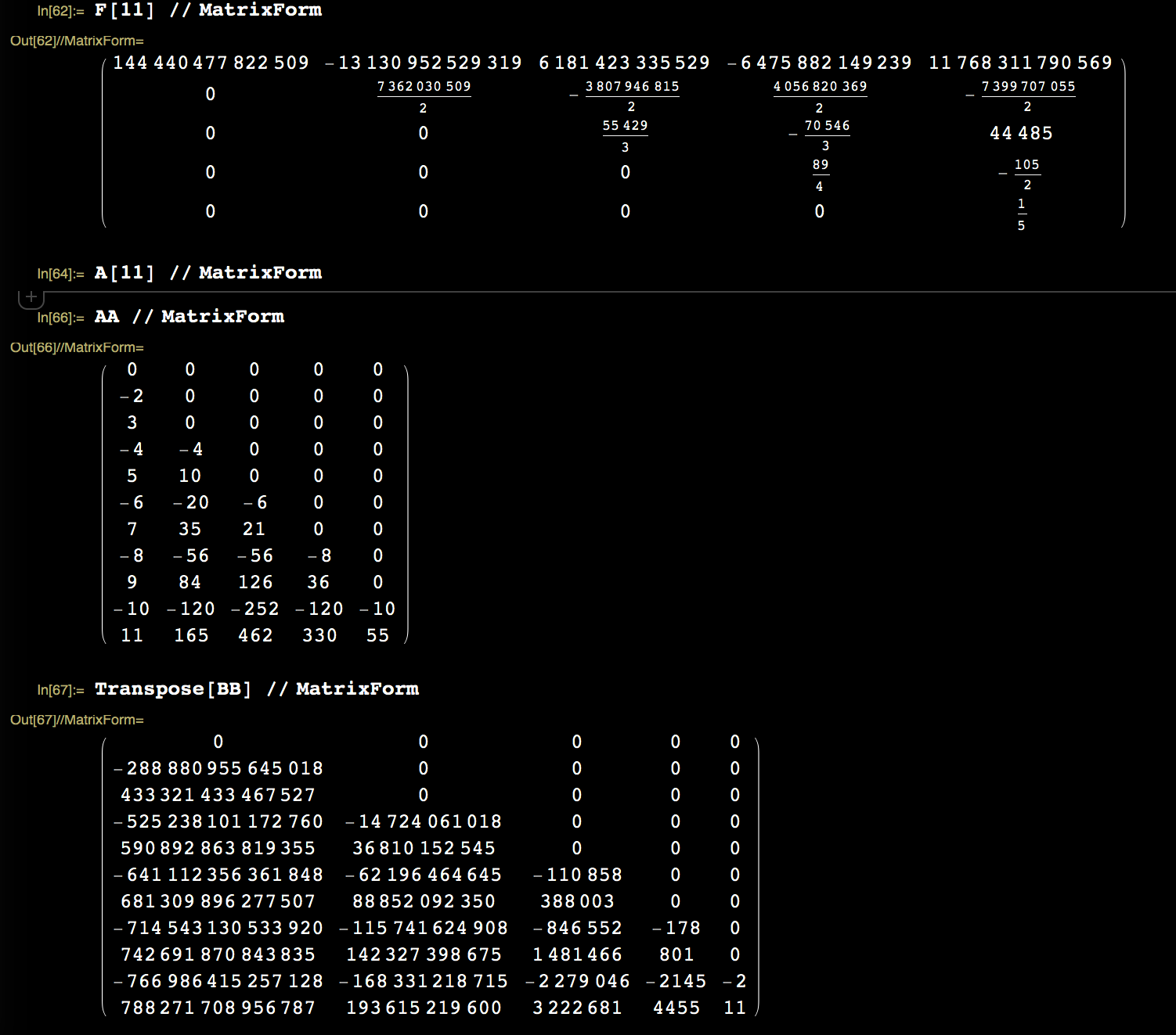
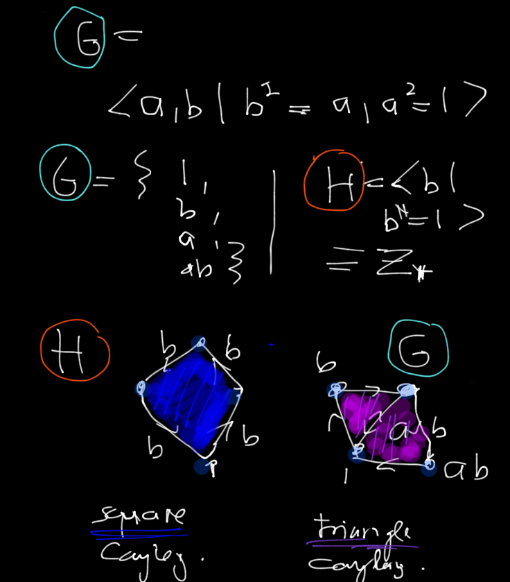
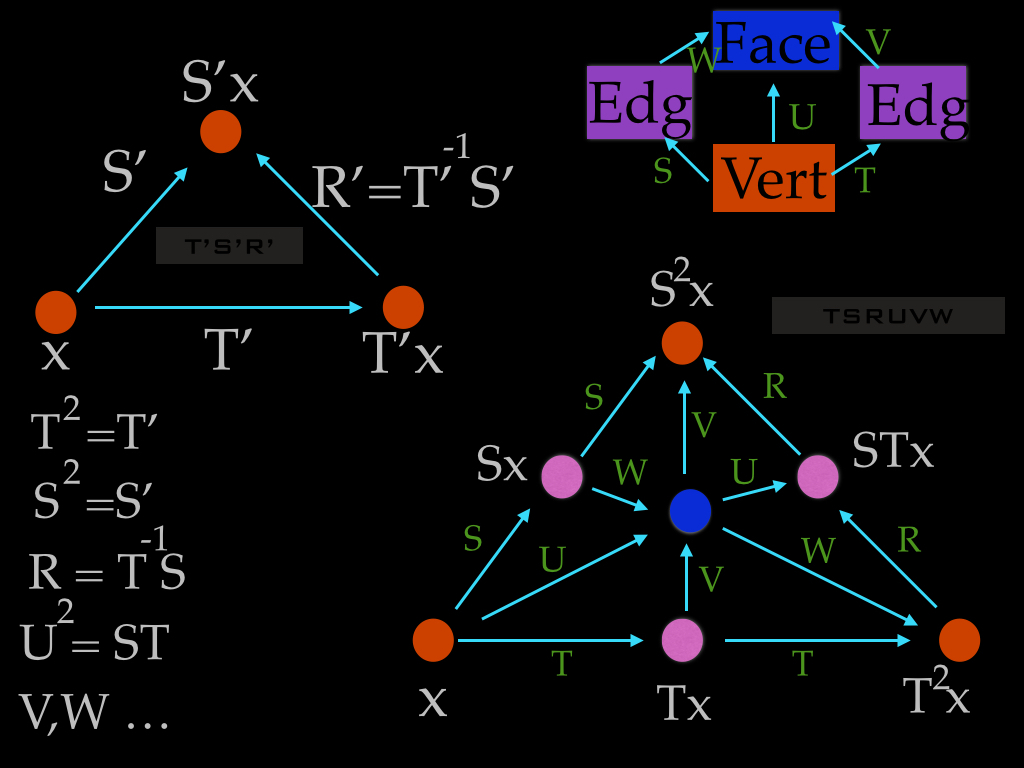
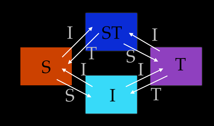 October 8: the limiting group in dimension d
can also be obtained from ergodic theory as the dyadic integers
can be constructed from within ergodic theory. I actually defined
the renormalization step as a graduate student already on the dynamical
level. I just did not look at the fixed point yet then. But it is the same
story as in one dimensions. As a group, the limiting space will be
the group D2d, the d'th direct product of the dyadic
group of integers. So, it is indeed again a profinite group as the product
of profinite groups is profinite.
Lets start with an arbitrary measure-preserving Zd action
on ([0,1],m) where m is the Lebesgue measure on the interval [0,1]. Again,
in the measure theoretical framework, taking the interval is not a loss of
generality, it is similar than using separable Hilbert spaces only).
Now take 2d copies of this interval and associate each interval with
a subset of I={1,...,d}. This gives 2d intervals.
Place the normalize Lebesgue measure on the union of the intervals.
Define a new Zd action by defining Ti
from an interval A to B if B = A u {i} to be the identity and
by defining Ti from A to B to be the old Ti
if B= A {i}. If the old dynamical system was a Zd
action, the new system is again a Zd action.
This multi-dimensional integral
extension of Zd actions was defined in
this paper [PDF].
In the same way than in 1 dimension, one can now define a uniform metric
on the set of all Zd actions on [0,1]. It is given by the distance d(T,S)
defined as the Lebesgue measure of all x for which one
Ti(x) disagrees with Si(x).
Again, this is a complete metric space and the integral extension
renormalization map is a contraction, as it halfs the distance between
two initial points in each step (after n steps, the maps agree on 1-2n of the interval.
The Koopman operator (U_1,...,U_d) on the product Hilbert space
L2(I) x ... x L2(I)
has again discrete product spectrum in T1 x ...xT1.
Each of the generators Ti has the dyadic complex numbers
exp(i k/2n) as eigenvalues of its Koopman unitary operator.
The limiting dynamical system is a uniquely ergodic Zd
action on the compact topological group D2d. Each
transformation generating the Zd action is almost periodic and isomorphic to
the adding machine on a quotient space similarly than any translation on Rd
is a translation on R when taking the quotient with the orthogonal complement of an
orbit. Next, we will have to realize the
Barycentric refinement inside this picture and then define the Laplacian, the
almost periodic random operator which is the Barycentric limit of Laplacians on graphs.
Here is an illustration from page 212 of my thesis which illustrates the convergence of the
renormalization map on dynamical systems in one dimensions leading to the piecewise
linear interval map called von Neumann-Kakutani system, which is the addition on the
dyadic group of integers. One can see graphically the selfsimilar structure and that
taking the return map onto one of the half intervals produces the same picture. This
picture does not do justice to the situation in higher dimensions as that one will be
much more rich.
October 8: the limiting group in dimension d
can also be obtained from ergodic theory as the dyadic integers
can be constructed from within ergodic theory. I actually defined
the renormalization step as a graduate student already on the dynamical
level. I just did not look at the fixed point yet then. But it is the same
story as in one dimensions. As a group, the limiting space will be
the group D2d, the d'th direct product of the dyadic
group of integers. So, it is indeed again a profinite group as the product
of profinite groups is profinite.
Lets start with an arbitrary measure-preserving Zd action
on ([0,1],m) where m is the Lebesgue measure on the interval [0,1]. Again,
in the measure theoretical framework, taking the interval is not a loss of
generality, it is similar than using separable Hilbert spaces only).
Now take 2d copies of this interval and associate each interval with
a subset of I={1,...,d}. This gives 2d intervals.
Place the normalize Lebesgue measure on the union of the intervals.
Define a new Zd action by defining Ti
from an interval A to B if B = A u {i} to be the identity and
by defining Ti from A to B to be the old Ti
if B= A {i}. If the old dynamical system was a Zd
action, the new system is again a Zd action.
This multi-dimensional integral
extension of Zd actions was defined in
this paper [PDF].
In the same way than in 1 dimension, one can now define a uniform metric
on the set of all Zd actions on [0,1]. It is given by the distance d(T,S)
defined as the Lebesgue measure of all x for which one
Ti(x) disagrees with Si(x).
Again, this is a complete metric space and the integral extension
renormalization map is a contraction, as it halfs the distance between
two initial points in each step (after n steps, the maps agree on 1-2n of the interval.
The Koopman operator (U_1,...,U_d) on the product Hilbert space
L2(I) x ... x L2(I)
has again discrete product spectrum in T1 x ...xT1.
Each of the generators Ti has the dyadic complex numbers
exp(i k/2n) as eigenvalues of its Koopman unitary operator.
The limiting dynamical system is a uniquely ergodic Zd
action on the compact topological group D2d. Each
transformation generating the Zd action is almost periodic and isomorphic to
the adding machine on a quotient space similarly than any translation on Rd
is a translation on R when taking the quotient with the orthogonal complement of an
orbit. Next, we will have to realize the
Barycentric refinement inside this picture and then define the Laplacian, the
almost periodic random operator which is the Barycentric limit of Laplacians on graphs.
Here is an illustration from page 212 of my thesis which illustrates the convergence of the
renormalization map on dynamical systems in one dimensions leading to the piecewise
linear interval map called von Neumann-Kakutani system, which is the addition on the
dyadic group of integers. One can see graphically the selfsimilar structure and that
taking the return map onto one of the half intervals produces the same picture. This
picture does not do justice to the situation in higher dimensions as that one will be
much more rich.
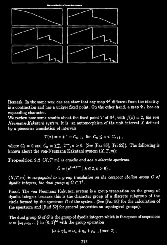


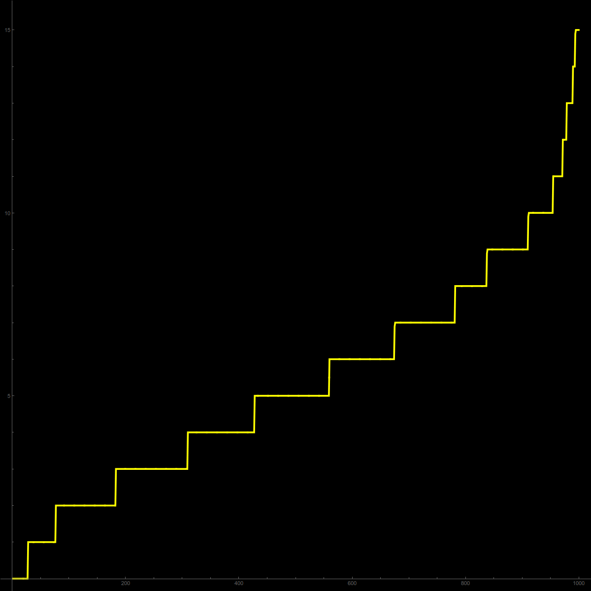
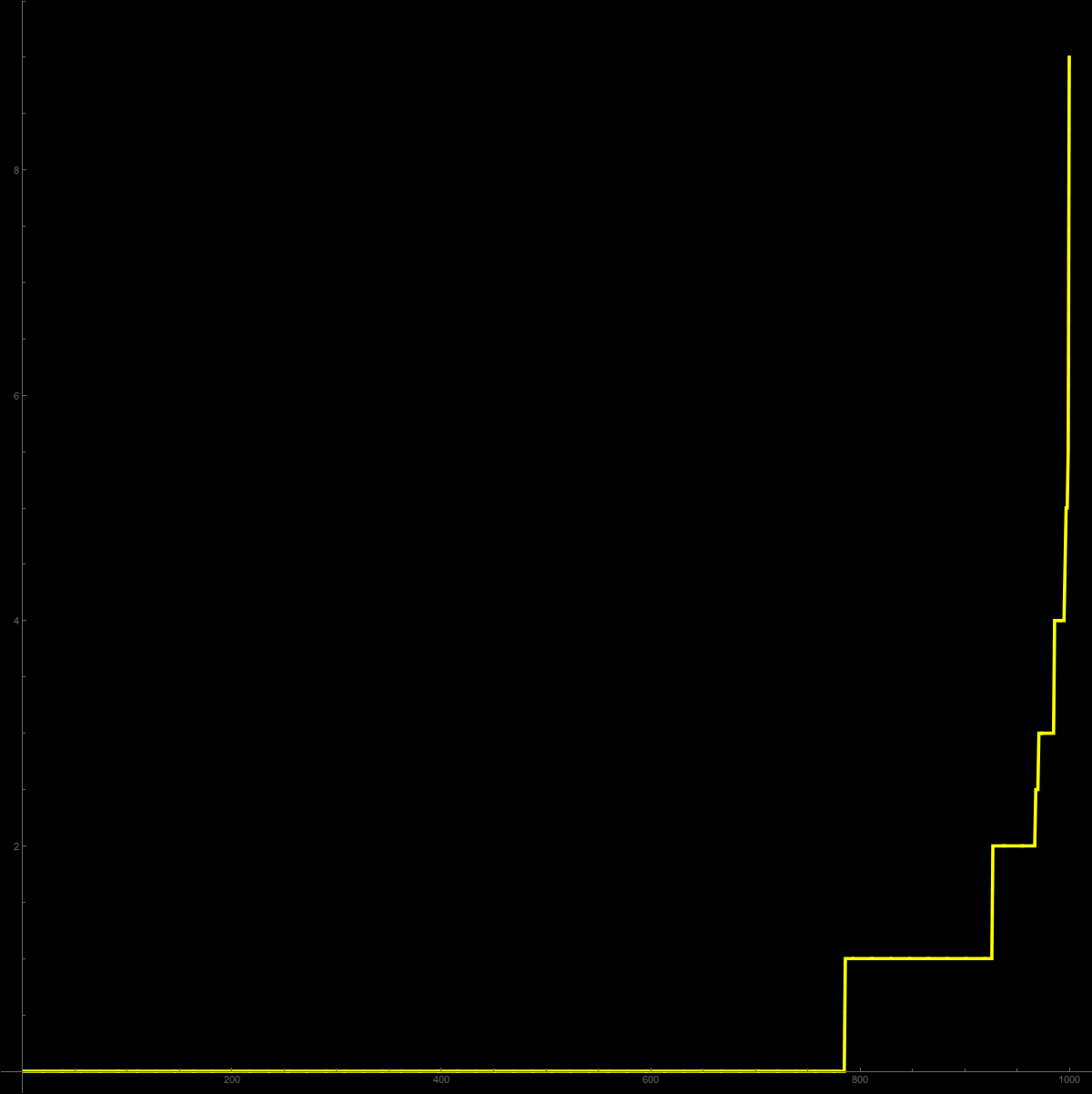


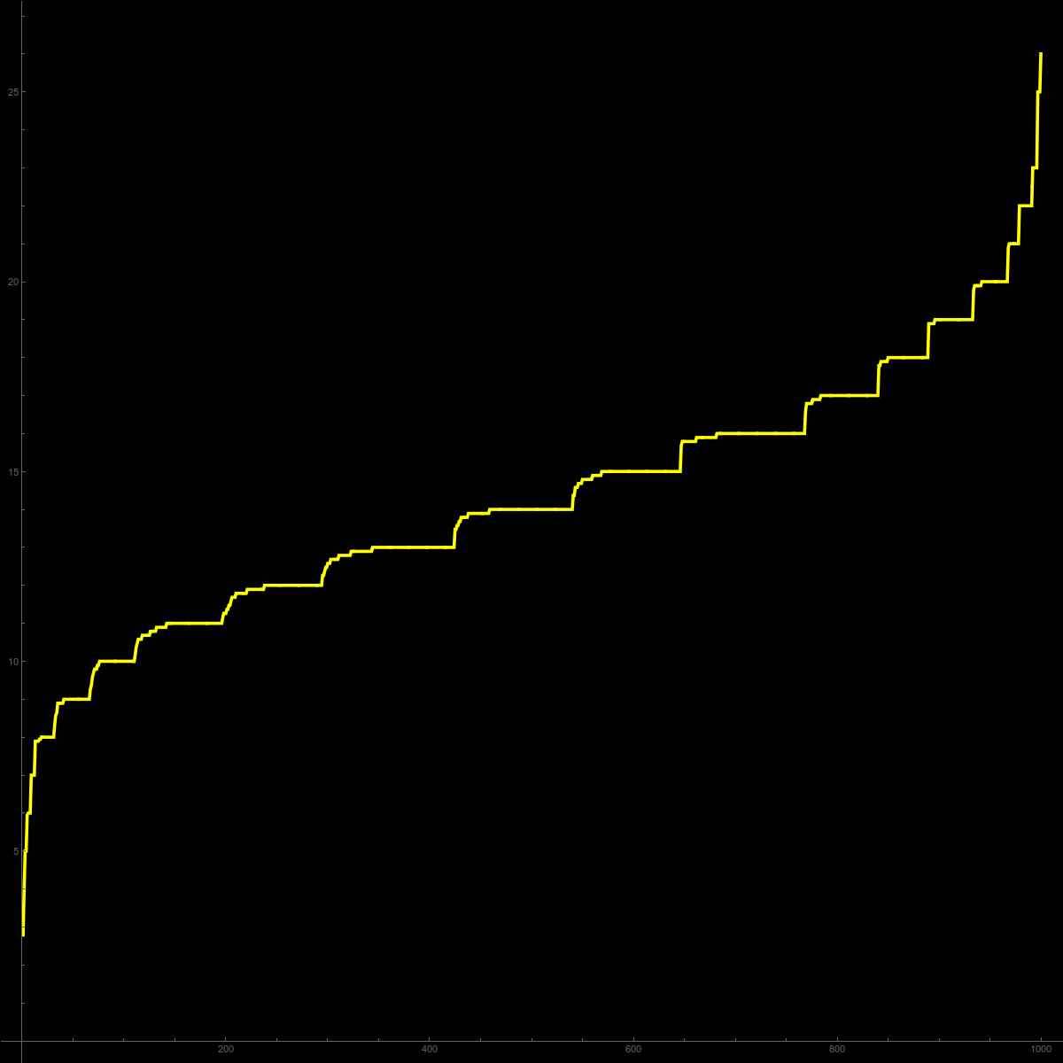
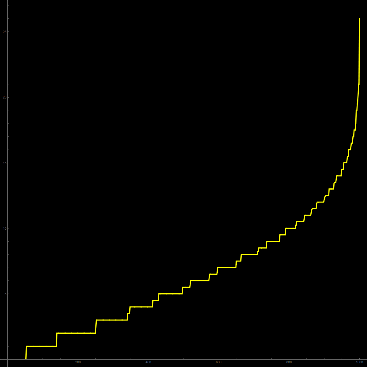


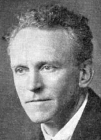
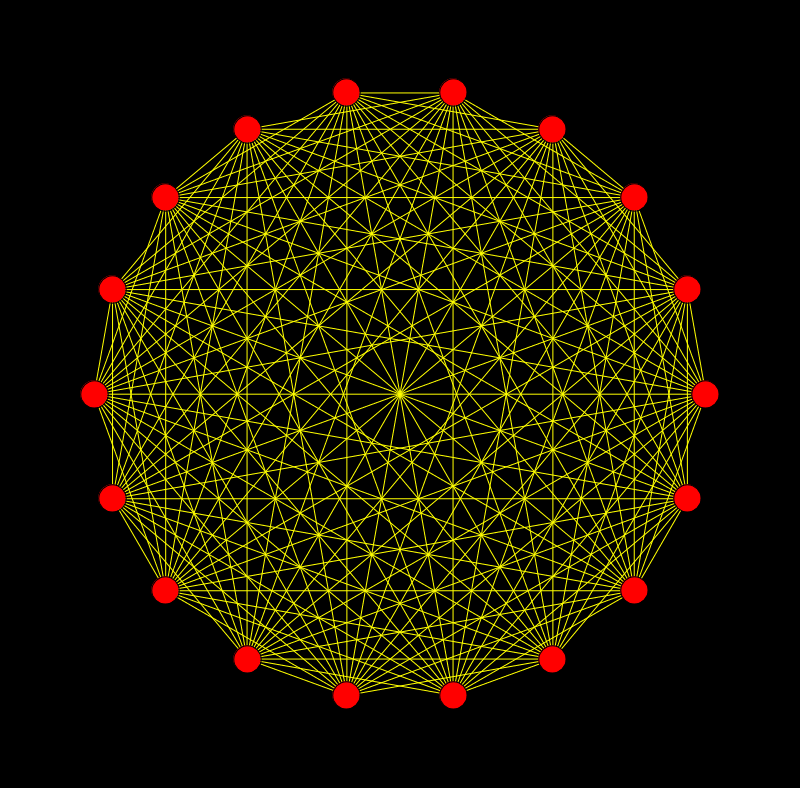 Lets look at at an 8 dimensional sphere G (the 8-dimensional octahedron). The graph is
shown in the picture. You see why graphs are nice. Unlike simplicial complexes which need
a considerable amount of math to even be defined, any kid can draw an 8 sphere: draw a circle,
place 18 points and connect any two dots, except dots which are opposite to each other.
This is an 8 dimensional Evako sphere: each unit sphere is a 7 sphere.
This 8-sphere has the clique data
Lets look at at an 8 dimensional sphere G (the 8-dimensional octahedron). The graph is
shown in the picture. You see why graphs are nice. Unlike simplicial complexes which need
a considerable amount of math to even be defined, any kid can draw an 8 sphere: draw a circle,
place 18 points and connect any two dots, except dots which are opposite to each other.
This is an 8 dimensional Evako sphere: each unit sphere is a 7 sphere.
This 8-sphere has the clique data
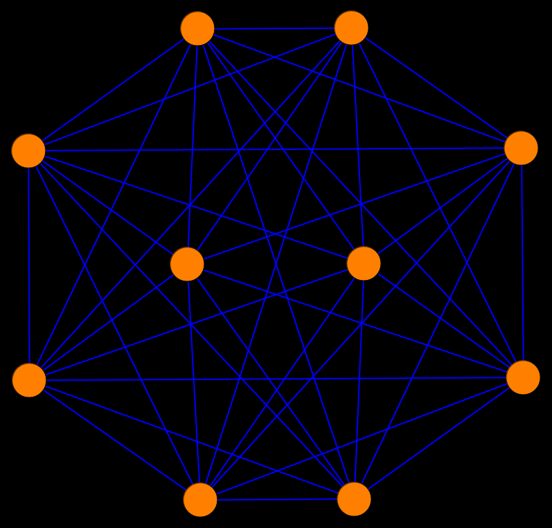 Very exciting: for even dimensional 2d-graphs (graphs for which the unit spheres are
(2d-1)-spheres), the eigenfunctions f2k of the Barycentric operator AT lead to
new invariants. The first new case is for 4-graphs = discrete 4 manifolds which appear for example for
nice triangulations of real 4 manifolds. Lets take a 4-sphere:
with clique vector v=(10,40,80,80,32). The eigenvectors of AT restricted to 4-graphs are
(0, 0, 0, 0, 1),(0, 0, 0, -2, 5),(0, 0, 19, -38, 55), (0, -22, 33, -40, 45),(1, -1, 1, -1, 1),
where the first is volume and the last is the well known Euler characteristic.
The second and fourth vectors are perpendicular to the clique vector.
Very exciting: for even dimensional 2d-graphs (graphs for which the unit spheres are
(2d-1)-spheres), the eigenfunctions f2k of the Barycentric operator AT lead to
new invariants. The first new case is for 4-graphs = discrete 4 manifolds which appear for example for
nice triangulations of real 4 manifolds. Lets take a 4-sphere:
with clique vector v=(10,40,80,80,32). The eigenvectors of AT restricted to 4-graphs are
(0, 0, 0, 0, 1),(0, 0, 0, -2, 5),(0, 0, 19, -38, 55), (0, -22, 33, -40, 45),(1, -1, 1, -1, 1),
where the first is volume and the last is the well known Euler characteristic.
The second and fourth vectors are perpendicular to the clique vector.
 The second is the trivial handshake invariant. The fourth leads to a new Barycentric invariant
which I have never seen:
The second is the trivial handshake invariant. The fourth leads to a new Barycentric invariant
which I have never seen:
 This functional on 4-graphs remains zero also after edge subdivisions (which I used for
graph coloring embeddings).
For example, after 10 random edge refinements, we get a deformed
4-sphere with data (20, 115, 280, 305, 122). It is perpendicular to (0, -22, 33, -40, 45) leading
to X(G)=0.
Also the clique data of the Barycentric refinement G1 which are (842, 9840, 30960, 36600, 14640)
satisfies this by definition. The invariant appears to be zero for all 4-graphs independent of
its topology.
Here is an other example graph G=S2 x S2 with
Clique data of G are (196, 2304, 7296, 8640, 3456) and Euler characteristic
chi(G) = 196 - 2304 + 7296 - 8640 + 3456=4. We see that the
graph product is handy for constructing
examples. Before I had the graph product, I had to construct such examples by hand, now
its for free. Also here, the mystery invariant is zero: X(G)=0.
More examples:
This functional on 4-graphs remains zero also after edge subdivisions (which I used for
graph coloring embeddings).
For example, after 10 random edge refinements, we get a deformed
4-sphere with data (20, 115, 280, 305, 122). It is perpendicular to (0, -22, 33, -40, 45) leading
to X(G)=0.
Also the clique data of the Barycentric refinement G1 which are (842, 9840, 30960, 36600, 14640)
satisfies this by definition. The invariant appears to be zero for all 4-graphs independent of
its topology.
Here is an other example graph G=S2 x S2 with
Clique data of G are (196, 2304, 7296, 8640, 3456) and Euler characteristic
chi(G) = 196 - 2304 + 7296 - 8640 + 3456=4. We see that the
graph product is handy for constructing
examples. Before I had the graph product, I had to construct such examples by hand, now
its for free. Also here, the mystery invariant is zero: X(G)=0.
More examples:
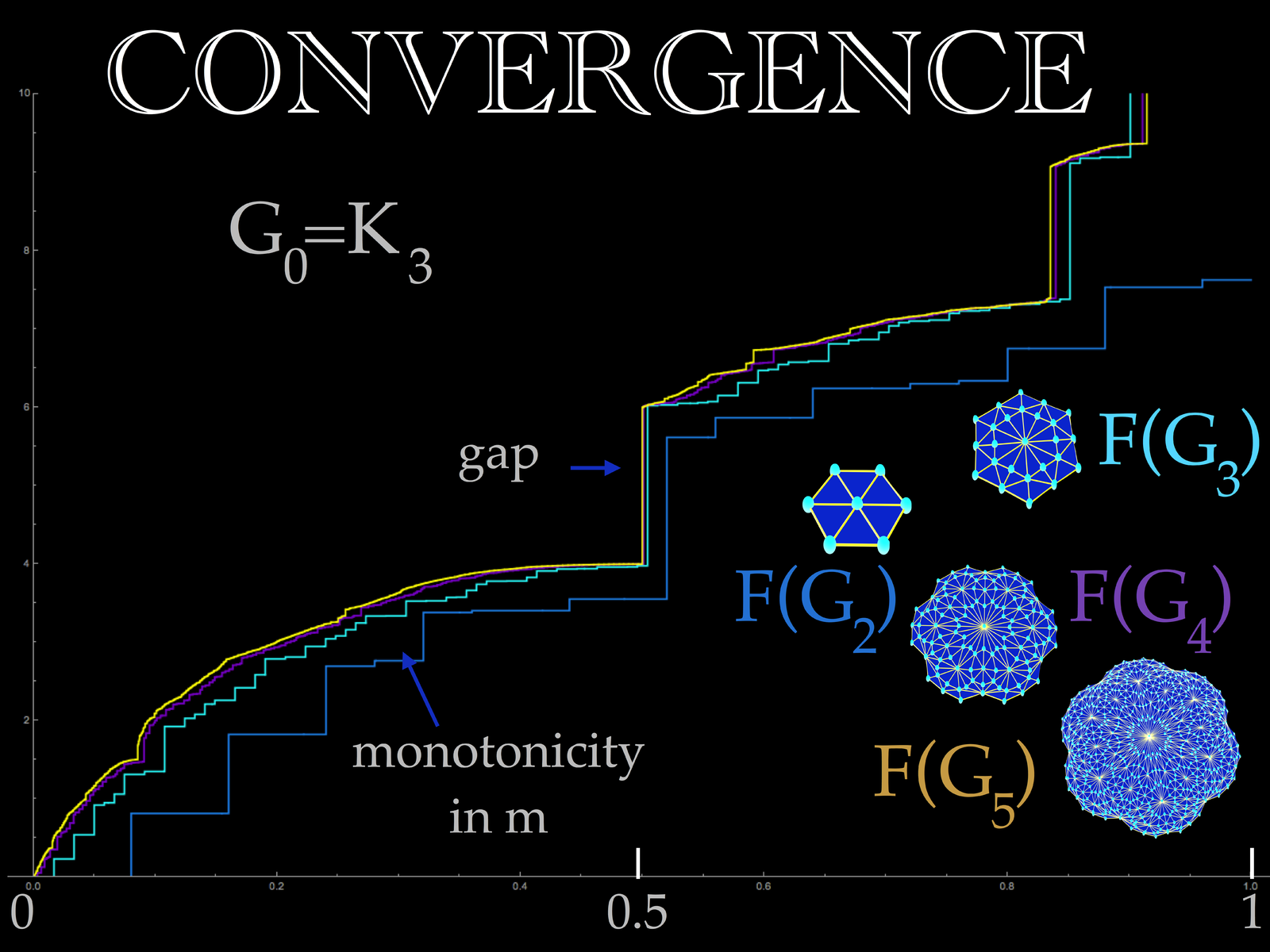
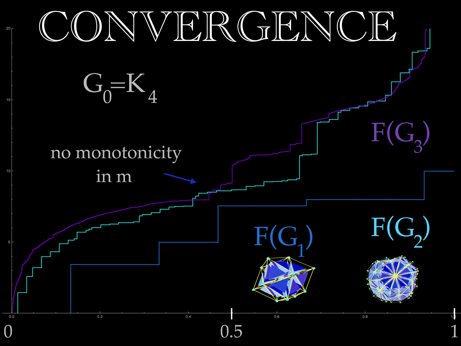

 August 24, 2015: what is the best Weyl asymptotic analog? One could look
for a graph with n vertices and maximal eigenvalue lambda(n), one could look at
the Weyl volume
August 24, 2015: what is the best Weyl asymptotic analog? One could look
for a graph with n vertices and maximal eigenvalue lambda(n), one could look at
the Weyl volume
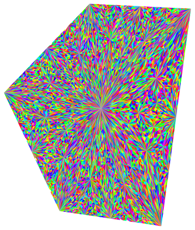 Just programmed Barycentric refinement also in Euclidean setting
(which does not need graph theory and is the usual setting.
See picture. We defined the Barycentric refinement
for any finite simple graph G as follows:
Just programmed Barycentric refinement also in Euclidean setting
(which does not need graph theory and is the usual setting.
See picture. We defined the Barycentric refinement
for any finite simple graph G as follows: 